# paquetes ----------------------------------------------------------------
library(glue)
library(ggtext)
library(showtext)
library(tidyverse)
# fuente ------------------------------------------------------------------
# colores
c1 <- "#0D2D4C"
c2 <- "#D0C8C1"
c3 <- "#F6F2EE"
c4 <- "#FD6E89"
c5 <- "#55092A"
c6 <- "black"
# fuente: Ubuntu
font_add(
family = "ubuntu",
regular = "fuente/Ubuntu-Regular.ttf",
bold = "fuente/Ubuntu-Bold.ttf",
italic = "fuente/Ubuntu-Italic.ttf")
# monoespacio & íconos
font_add(
family = "jet",
regular = "fuente/JetBrainsMonoNLNerdFontMono-Regular.ttf")
# bebas neue
font_add(
family = "bebas",
regular = "fuente/BebasNeue-Regular.ttf")
showtext_auto()
showtext_opts(dpi = 300)
# caption
fuente <- glue(
"Datos: <span style='color:{c4};'><span style='font-family:jet;'>",
"{{<b>tidytuesdayR</b>}}</span> semana {29}, ",
"<b>The English Women's Football Database</b>.</span>")
autor <- glue("<span style='color:{c4};'>**Víctor Gauto**</span>")
icon_twitter <- glue("<span style='font-family:jet;'></span>")
icon_instagram <- glue("<span style='font-family:jet;'></span>")
icon_github <- glue("<span style='font-family:jet;'></span>")
icon_mastodon <- glue("<span style='font-family:jet;'>󰫑</span>")
usuario <- glue("<span style='color:{c4};'>**vhgauto**</span>")
sep <- glue("**|**")
mi_caption <- glue(
"{fuente}<br>{autor} {sep} {icon_github} {icon_twitter} {icon_instagram} ",
"{icon_mastodon} {usuario}")
# datos -------------------------------------------------------------------
tuesdata <- tidytuesdayR::tt_load(2024, 29)
ewf_matches <- tuesdata$ewf_matches
# me interesa la popularidad anual de la asistencia a los estadios, y marcar
# el equipo más popular anual
d <- ewf_matches |>
mutate(año = year(date)) |>
select(año, attendance) |>
drop_na()
# medianas anuales
d_m <- d |>
reframe(
m = median(attendance),
.by = año
)
# equipo más convocante por año
tops <- ewf_matches |>
mutate(año = year(date)) |>
slice_max(order_by = attendance, by = año, n = 1) |>
select(año, home_team_name, attendance)
# combino datos
d2 <- full_join(d, tops, by = join_by(año, attendance)) |>
mutate(home_team_name = if_else(
is.na(home_team_name),
"Otros",
home_team_name
)
) |>
mutate(home_team_name = fct_reorder(home_team_name, attendance)) |>
mutate(home_team_name = fct_rev(home_team_name))
# figura ------------------------------------------------------------------
# paleta de colores
pal <- c(MoMAColors::moma.colors(palette_name = "Klein", n = 7), c2)
# cantidad de público en todo 2023
attendance_2023 <- ewf_matches |>
filter(year(date) == 2023) |>
reframe(
s = sum(attendance, na.rm = TRUE)
) |>
pull() |>
format(big.mark = ".", decimal.mark = ",")
# subtítulo
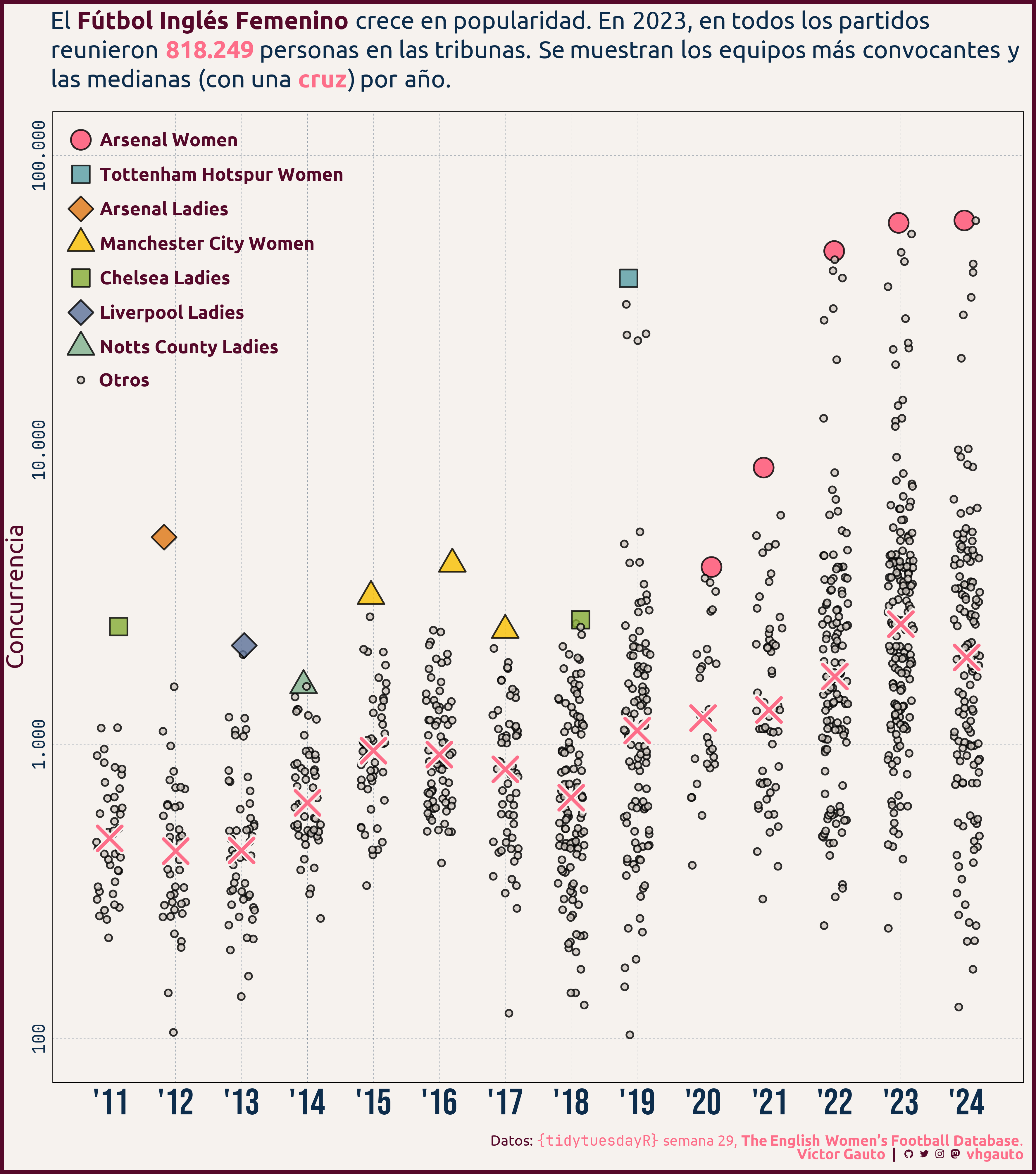
mi_subtitle <- glue(
"El <b style='color: {c5}'>Fútbol Inglés Femenino</b> crece en",
"popularidad. En 2023,",
"en todos los partidos reunieron <b style='color:{c4}'>{attendance_2023}</b>",
"personas en las tribunas. Se muestran los equipos más convocantes y las",
"medianas (con una <b style='color: {c4}'>cruz</b>) por año.",
.sep = " "
)
# figura
g <- ggplot(
d2, aes(
año, attendance, fill = home_team_name, shape = home_team_name,
size = home_team_name)) +
# puntos
geom_point(
alpha = .8, position = position_jitter(seed = 2024, width = .2), stroke = 1,
color = c6) +
# mediana
geom_point(
data = d_m, aes(año, m), fill = NA, color = c3, size = 7,
inherit.aes = FALSE, shape = 4, stroke = 4) +
geom_point(
data = d_m, aes(año, m), fill = NA, color = c4, size = 8,
inherit.aes = FALSE, shape = 4, stroke = 2) +
scale_x_continuous(breaks = 2011:2024, labels = glue("'{11:24}")) +
scale_y_log10(
breaks = 10^(2:5), limits = c(100, 1e5),
labels = c("100", "1.000", "10.000", "100.000")) +
scale_fill_manual(values = pal) +
scale_shape_manual(values = c(21:24, 22:24, 21)) +
scale_size_manual(values = c(rep(7, 7), 2)) +
labs(
x = NULL, y = "Concurrencia", fill = NULL, shape = NULL, size = NULL,
subtitle = mi_subtitle, caption = mi_caption) +
guides(
fill = guide_legend(position = "inside")
) +
theme_linedraw() +
theme(
aspect.ratio = 1,
plot.margin = margin(t = 5, l = 5, r = 10, b = 5),
plot.background = element_rect(fill = c3, color = c5, linewidth = 3),
plot.subtitle = element_textbox_simple(
family = "ubuntu", size = 20, margin = margin(b = 16, t = 5), color = c1),
plot.caption = element_markdown(
family = "ubuntu", size = 12, margin = margin(t = 15, b = 5), color = c5),
panel.background = element_blank(),
panel.grid.minor = element_blank(),
axis.ticks = element_blank(),
axis.text.x = element_text(family = "bebas", size = 30, color = c1),
panel.grid.major = element_line(linetype = "FF", color = c1),
axis.text.y = element_text(
family = "jet", size = 14, angle = 90, hjust = .5, color = c1),
axis.title.y = element_text(
family = "ubuntu", size = 20, color = c5),
legend.text = element_text(
size = 15, family = "ubuntu", face = "bold", color = c5),
legend.position.inside = c(.01, .99),
legend.background = element_rect(fill = NA),
legend.justification.inside = c(0, 1),
legend.key.spacing.y = unit(.3, "cm")
)
# guardo
ggsave(
plot = g,
filename = "2024/s29/viz.png",
width = 30,
height = 34,
units = "cm")
# abro
browseURL("2024/s29/viz.png")