Ocultar código
library(glue)
library(ggtext)
library(showtext)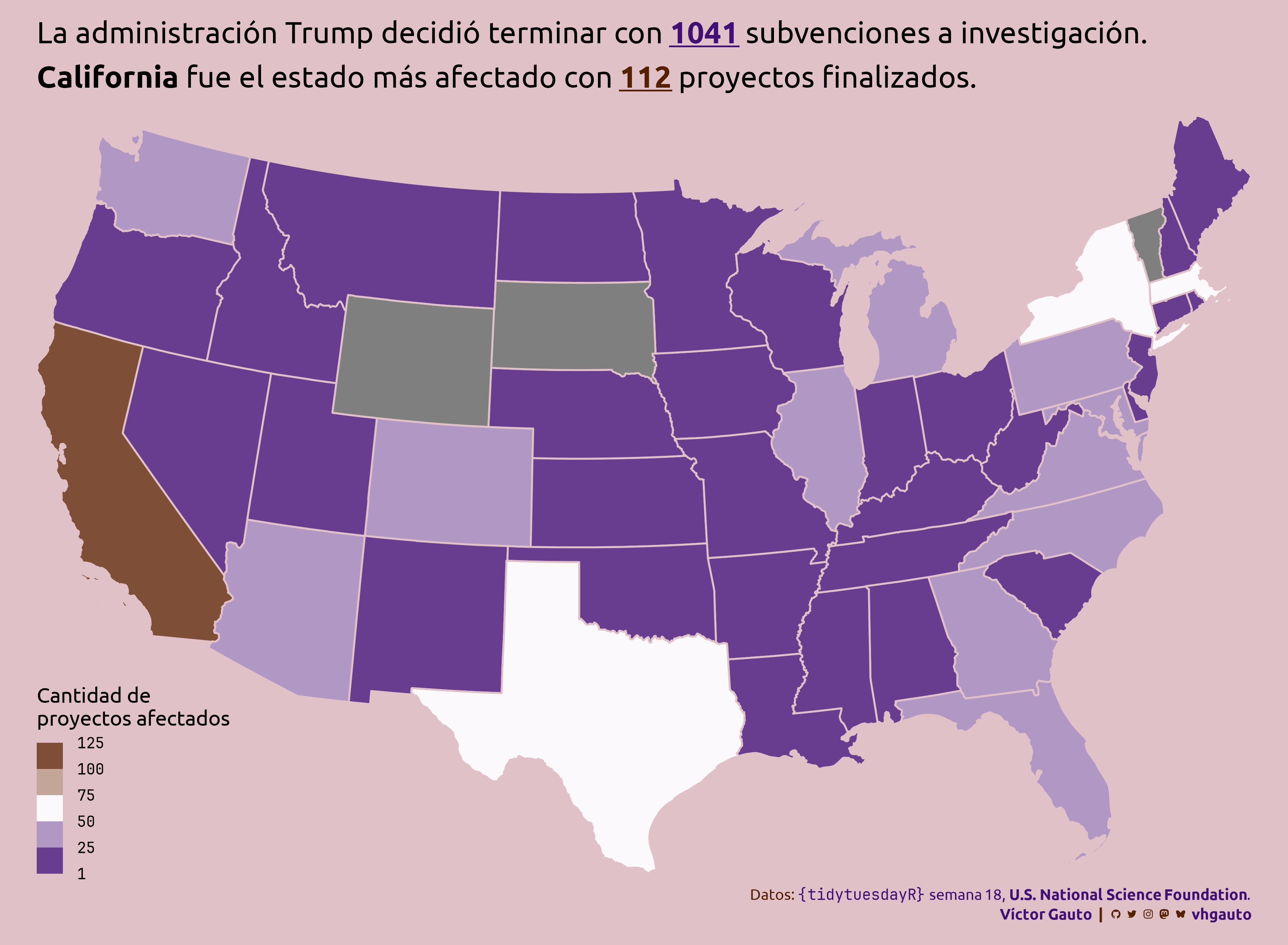
library(tidyverse)Cantidad de proyectos de investigación finalizados por estado en EE.UU.
library(glue)
library(ggtext)
library(showtext)
library(tidyverse)Colores.
c1 <- "#420F75"
c2 <- "#552000"
c3 <- "white"
c4 <- "#E1C1C8"
Fuentes: Ubuntu y JetBrains Mono.
font_add(
  family = "ubuntu",
  regular = "././fuente/Ubuntu-Regular.ttf",
  bold = "././fuente/Ubuntu-Bold.ttf",
  italic = "././fuente/Ubuntu-Italic.ttf"
)

font_add(
  family = "jet",
  regular = "././fuente/JetBrainsMonoNLNerdFontMono-Regular.ttf"
)

showtext_auto()
showtext_opts(dpi = 300)fuente <- glue(
"Datos: <span style='color:{c1};'><span style='font-family:jet;'>",
"{{<b>tidytuesdayR</b>}}</span> semana 18, ",
"<b>U.S. National Science Foundation</b>.</span>"
)
autor <- glue("<span style='color:{c1};'>**Víctor Gauto**</span>")
icon_twitter <- glue("<span style='font-family:jet;'></span>")
icon_instagram <- glue("<span style='font-family:jet;'></span>")
icon_github <- glue("<span style='font-family:jet;'></span>")
icon_mastodon <- glue("<span style='font-family:jet;'>󰫑</span>")
icon_bsky <- glue("<span style='font-family:jet;'></span>")
usuario <- glue("<span style='color:{c1};'>**vhgauto**</span>")
sep <- glue("**|**")
mi_caption <- glue(
"{fuente}<br>{autor} {sep} {icon_github} {icon_twitter} {icon_instagram} ",
"{icon_mastodon} {icon_bsky} {usuario}"
)tuesdata <- tidytuesdayR::tt_load(2025, 18)
nsf_terminations <- tuesdata$nsf_terminationsMe interesa ver la distribución de proyectos cancelados por estado de EE.UU, mediante un mapa.
d <- nsf_terminations |>
  count(org_state) |>
rename(state = org_state)Subtítulo indicando la cantidad de proyectos afectados y el estado con mayor cantidad.
mi_subtitulo <- glue(
  "La administración Trump decidió terminar con {{{c1} _**{nrow(nsf_terminations)}**_}
  subvenciones a investigación.
  **California** fue el estado más afectado con {{{c2} _**{d[d$n == max(d$n),]$n}**_} proyectos finalizados."
)g <- usmap::plot_usmap(
exclude = c("AK", "HI"),
data = d,
values = "n",
color = c4,
linewidth = .6
) +
coord_sf(expand = FALSE) +
scale_fill_steps2(
low = c1,
mid = c3,
high = c2,
midpoint = 64,
breaks = c(1, seq(25, 125, 25)),
limits = c(1, 125)
) +
labs(
subtitle = mi_subtitulo,
fill = "Cantidad de\nproyectos afectados",
caption = mi_caption
) +
theme_void(base_family = "ubuntu", base_size = 20) +
theme(
plot.margin = margin(t = 10, b = 5, r = 15, l = 15),
plot.background = element_rect(fill = c4, color = NA),
plot.subtitle = marquee::element_marquee(
width = .92, lineheight = 1.3, size = rel(1.), margin = margin(b = 15)
),
plot.caption = element_markdown(
color = c2, size = rel(.5), margin = margin(b = 10, t = 10),
lineheight = 1.3
),
legend.position = "inside",
legend.position.inside = c(0, 0),
legend.justification.inside = c(0, 0),
legend.title = element_text(size = rel(.7)),
legend.text = element_text(family = "jet", size = rel(.5))
)Guardo.
ggsave(
  plot = g,
  filename = "tidytuesday/2025/semana_18.png",
  width = 30,
  height = 22,
  units = "cm"
)