Ocultar código
library(glue)
library(ggtext)
library(showtext)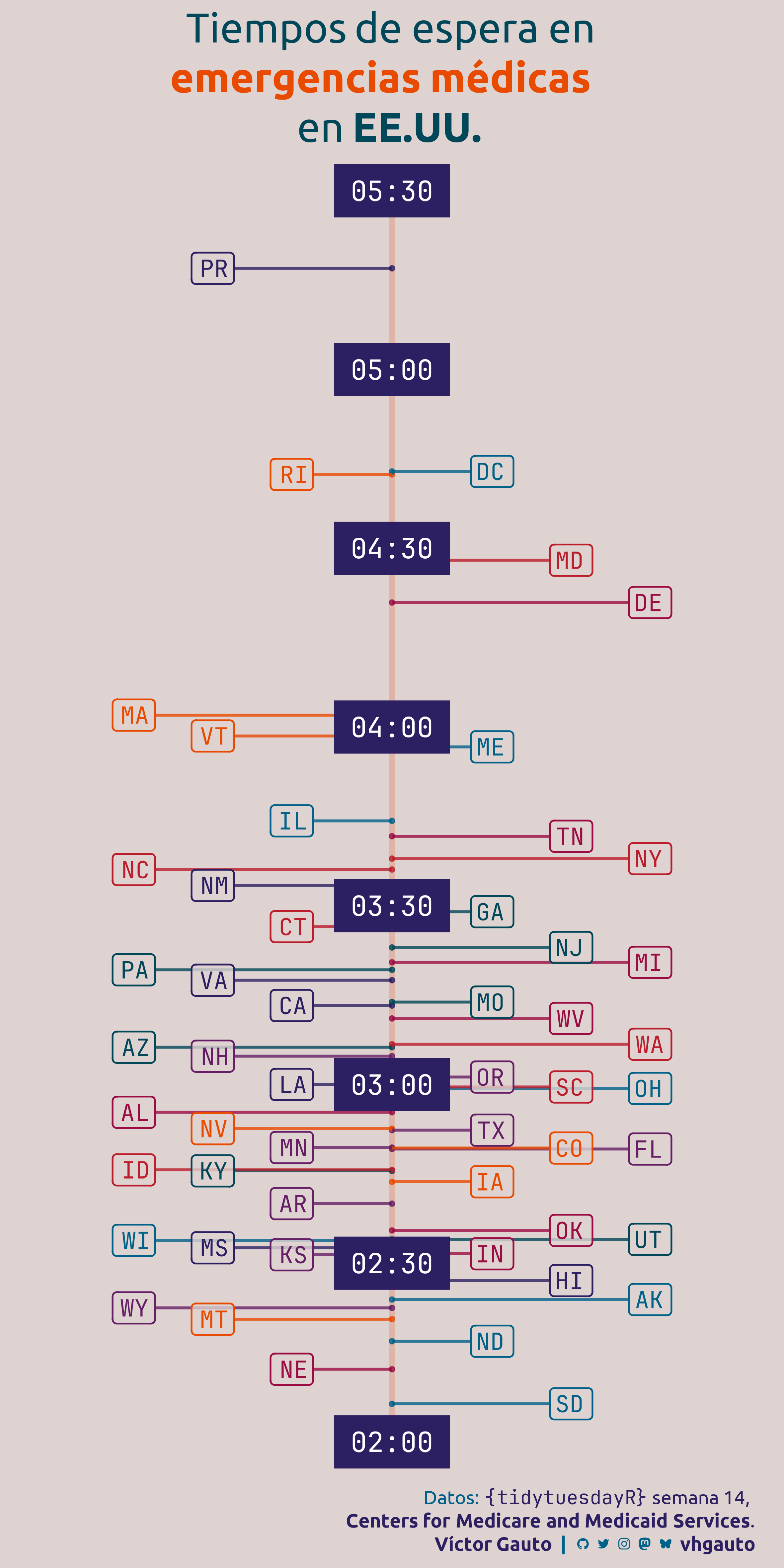
library(tidyverse)Tiempo de espera en EE.UU. en caso de atención de una emergencia médica.
library(glue)
library(ggtext)
library(showtext)
library(tidyverse)Colores.
col <- MoMAColors::moma.colors(palette_name = "Panton", 7)
c1 <- "#DFD3D1"
c2 <- "#DFAE9C"
Fuentes: Ubuntu y JetBrains Mono.
font_add(
  family = "ubuntu",
  regular = "././fuente/Ubuntu-Regular.ttf",
  bold = "././fuente/Ubuntu-Bold.ttf",
  italic = "././fuente/Ubuntu-Italic.ttf"
)

font_add(
  family = "jet",
  regular = "././fuente/JetBrainsMonoNLNerdFontMono-Regular.ttf"
)

showtext_auto()
showtext_opts(dpi = 300)fuente <- glue(
"Datos: <span style='color:{col[5]};'><span style='font-family:jet;'>",
"{{<b>tidytuesdayR</b>}}</span> semana 14, ",
"<b><br>Centers for Medicare and Medicaid Services</b>.</span>"
)
autor <- glue("<span style='color:{col[5]};'>**Víctor Gauto**</span>")
icon_twitter <- glue("<span style='font-family:jet;'></span>")
icon_instagram <- glue("<span style='font-family:jet;'></span>")
icon_github <- glue("<span style='font-family:jet;'></span>")
icon_mastodon <- glue("<span style='font-family:jet;'>󰫑</span>")
icon_bsky <- glue("<span style='font-family:jet;'></span>")
usuario <- glue("<span style='color:{col[5]};'>**vhgauto**</span>")
sep <- glue("**|**")
mi_caption <- glue(
"{fuente}<br>{autor} {sep} {icon_github} {icon_twitter} {icon_instagram} ",
"{icon_mastodon} {icon_bsky} {usuario}"
)tuesdata <- tidytuesdayR::tt_load(2025, 14)
care_state <- tuesdata$care_stateMe interesa agrupar los estados por tiempo promedio de espera en caso de emergencias.
Los colores se asignan aleatoriamente.
set.seed(111)

d <- care_state |>
  filter(condition == "Emergency Department") |>
  select(state, score) |>
  reframe(
    m = mean(score, na.rm = TRUE),
    .by = state
  ) |>
  mutate(tiempo = hms::hms(minute = m)) |>
  mutate(
    hora = hour(tiempo),
    minuto = minute(tiempo)
  ) |>
  mutate(label = paste0(hora, "H ", minuto, "M")) %>%
  mutate(
    col = rep(sample(col), length.out = nrow(.))
)Etiquetas del tiempo de espera en el centro de la figura. Agrego subtítulo y nivel de transparencia.
eje_v <- map(
  .x = 0:7,
  ~hms::hms(period(c(2, 30*.x), c("hour", "minute")))
) |>
  list_c()

eje_v_label <- paste0(
  "0",
  hour(eje_v), ":",
  if_else(minute(eje_v) == 0, "00", as.character(minute(eje_v)))
)

mi_subtitulo <- glue(
  "Tiempos de espera en<br><b style='color: {col[1]}'>emergencias médicas</b>
  <br>en **EE.UU.**"
)

alfa <- .8
Figura.
g <- d |>
  arrange(tiempo) %>%
  mutate(
    x = rep(sample(c(-3:-1, 1:3)), length.out = nrow(.))
  ) |>
  mutate(
    hjust = if_else(x < 0, 1, 0)
  ) |>
  ggplot(aes(0, tiempo, color = col)) +
  geom_vline(
    xintercept = 0, linewidth = 2, linetype = 1, color = c2, alpha = alfa
  ) +
  geom_point(alpha = alfa) +
  geom_segment(
    aes(x = 0, xend = x), alpha = alfa, linewidth = 1
  ) +
  geom_label(
    aes(x = x, label = state, hjust = hjust), size = 6, family = "jet",
    fill = alpha(c1, alfa), label.size = .6
  ) +
  annotate(
    geom = "label", x = 0, y = eje_v, label = eje_v_label, fill = col[5],
    label.size = unit(0, "mm"), label.padding = unit(0.5, "lines"), size = 7,
    family = "jet", color = "white", label.r = unit(0, "mm")
  ) +
  scale_y_continuous(expand = c(0, 0)) +
  scale_color_identity() +
  coord_cartesian(clip = "off") +
  labs(
    subtitle = mi_subtitulo, caption = mi_caption
  ) +
  theme_void() +
  theme(
    aspect.ratio = 2.4,
    text = element_text(family = "ubuntu"),
    plot.background = element_rect(fill = c1, color = NA),
    plot.subtitle = element_markdown(
      color = col[7], size = 30, margin = margin(b = 30, t = 10), hjust = .5,
      lineheight = 1.2
    ),
    plot.caption = element_markdown(
      color = col[6], size = 14, margin = margin(t = 35, b = 10, r = -75),
      lineheight = 1.2
    ),
    panel.background = element_blank()
  )
Guardo.
ggsave(
  plot = g,
  filename = "tidytuesday/2025/semana_14.png",
  width = 20,
  height = 40,
  units = "cm"
)