Ocultar código
library(glue)
library(ggtext)
library(showtext)
library(tidyverse)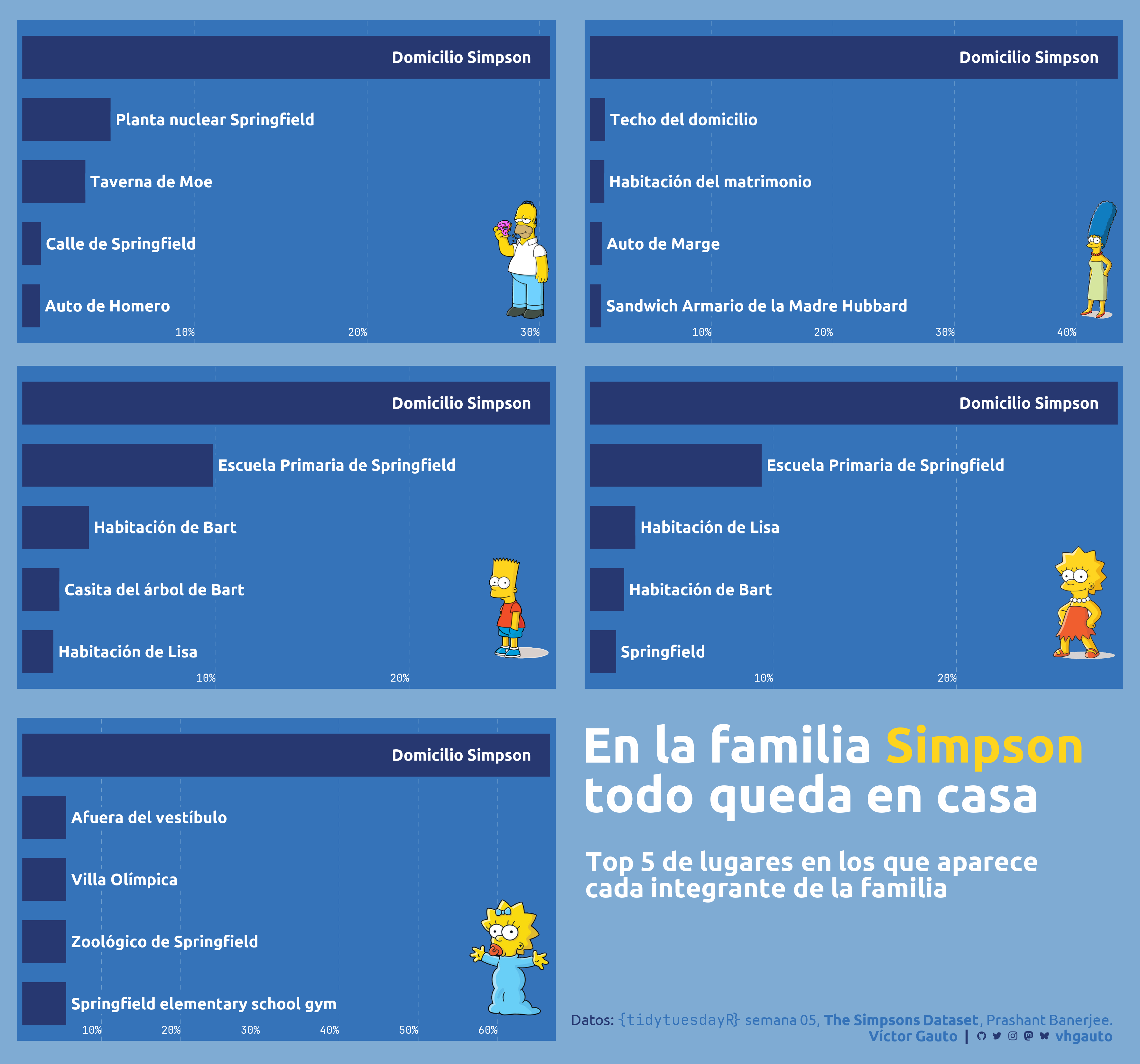
library(patchwork)Lugares más frecuentes de la familia Simpson.
library(glue)
library(ggtext)
library(showtext)
library(tidyverse)
library(patchwork)Colores
c1 <- "#7FABD3"
c2 <- "#3573B9"
c3 <- "#273871"
c4 <- "#FED41D"
c5 <- "white"
Fuentes: Ubuntu y JetBrains Mono
font_add(
  family = "ubuntu",
  regular = "././fuente/Ubuntu-Regular.ttf",
  bold = "././fuente/Ubuntu-Bold.ttf",
  italic = "././fuente/Ubuntu-Italic.ttf"
)

font_add(
  family = "jet",
  regular = "././fuente/JetBrainsMonoNLNerdFontMono-Regular.ttf"
)

showtext_auto()
showtext_opts(dpi = 300)fuente <- glue(
"Datos: <span style='color:{c2};'><span style='font-family:jet;'>",
"{{<b>tidytuesdayR</b>}}</span> semana 05, ",
"<b>The Simpsons Dataset</b>, Prashant Banerjee.</span>"
)
autor <- glue("<span style='color:{c2};'>**Víctor Gauto**</span>")
icon_twitter <- glue("<span style='font-family:jet;'></span>")
icon_instagram <- glue("<span style='font-family:jet;'></span>")
icon_github <- glue("<span style='font-family:jet;'></span>")
icon_mastodon <- glue("<span style='font-family:jet;'>󰫑</span>")
icon_bsky <- glue("<span style='font-family:jet;'></span>")
usuario <- glue("<span style='color:{c2};'>**vhgauto**</span>")
sep <- glue("**|**")
mi_caption <- glue(
"{fuente}<br>{autor} {sep} {icon_github} {icon_twitter} {icon_instagram} ",
"{icon_mastodon} {icon_bsky} {usuario}"
)tuesdata <- tidytuesdayR::tt_load(2025, 05)
locations <- tuesdata$simpsons_locations
script_lines <- tuesdata$simpsons_script_linesMe interesa asociar lugares a los integrantes principales de la familia Simpson.
Creo un vector con los nombres y links a sus imágenes sacado de Wikipedia.
familia <- c(
  "Homer Simpson", "Lisa Simpson", "Bart Simpson", "Marge Simpson",
  "Maggie Simpson"
)

link_familia <- c(
  Homero = "https://upload.wikimedia.org/wikipedia/en/0/02/Homer_Simpson_2006.png",
  Marge = "https://upload.wikimedia.org/wikipedia/en/0/0b/Marge_Simpson.png",
  Bart = "https://upload.wikimedia.org/wikipedia/en/a/aa/Bart_Simpson_200px.png",
  Lisa = "https://upload.wikimedia.org/wikipedia/en/e/ec/Lisa_Simpson.png",
  Maggie = "https://upload.wikimedia.org/wikipedia/en/9/9d/Maggie_Simpson.png"
)

img_familia <- glue("<img src='{link_familia}' height=90 />") |>
  as.character()

img_familia <- set_names(img_familia, names(link_familia))
Filtro el dataset del guión obteniendo los 5 sitios más frecuentes por cada integrante.
d <- script_lines |>
  filter(raw_character_text %in% familia) |>
  count(raw_character_text, location_id) |>
  inner_join(locations, by = join_by(location_id == id)) |>
  select(!normalized_name) |>
  select(
    personaje = raw_character_text,
    lugar = name,
    n
  ) |>
  mutate(
    personaje = str_remove(personaje, " Simpson")
  ) |>
  mutate(
    personaje = if_else(personaje == "Homer", "Homero", personaje)
  ) |>
  mutate(
    personaje = fct(
      personaje, levels = c("Homero", "Marge", "Bart", "Lisa", "Maggie")
    )
  ) |>
  arrange(personaje, n) |>
  mutate(
    puesto = row_number(), .by = personaje
  ) |>
  arrange(personaje, puesto) |>
  mutate(
    p = n/sum(n),
    .by = personaje
  ) |>
  mutate(
    puesto = factor(puesto)
  ) |>
  mutate(
    img = img_familia[personaje]
  ) |>
  mutate(
    lugar = str_to_sentence(lugar)
  ) |>
  mutate(
    hjust = if_else(lugar == "Simpson home", 1.1, 0)
  ) |>
  mutate(
    relleno = if_else(lugar == "Simpson home", c3, c2)
  ) |>
  slice_max(order_by = puesto, n = 5, by = personaje, with_ties = FALSE)
Traduzco los lugares
d <- d |>
  mutate(
    lugar = case_match(
      lugar,
      "Simpson home" ~ "Domicilio Simpson",
      "Springfield nuclear power plant" ~ "Planta nuclear Springfield",
      "Moe's tavern" ~ "Taverna de Moe",
      "Springfield street" ~ "Calle de Springfield",
      "Homer's car" ~ "Auto de Homero",
      "Evergreen terrace" ~ "Techo del domicilio",
      "Simpson master bedroom" ~ "Habitación del matrimonio",
      "Marge's car" ~ "Auto de Marge",
      "Mother hubbard's sandwich cupboard" ~ "Sandwich Armario de la Madre Hubbard",
      "Outer concourse" ~ "Afuera del vestíbulo",
      "Olympic village" ~ "Villa Olímpica",
      "First church of springfield" ~ "1ra Iglesia de Springfield",
      "Springfield elementary school" ~ "Escuela Primaria de Springfield",
      "Bart's bedroom" ~ "Habitación de Bart",
      "Bart's treehouse" ~ "Casita del árbol de Bart",
      "Lisa's bedroom" ~ "Habitación de Lisa",
      "Parking structure" ~ "Estacionamiento",
      "Springfield zoo" ~ "Zoológico de Springfield",
      .default = lugar
    )
)Genero un tibble para las etiquetas del eje horizontal.
eje_x <- tibble(
  x = seq(.1, .7, .1), y = .5
) |>
  mutate(
    label = paste0(x*100, "%")
  )
Figura principal.
g <- ggplot(d, aes(p, puesto)) +
  geom_segment(
    aes(x = 0, xend = p, yend = puesto), linewidth = 15, color = c3
  ) +
  geom_label(
    aes(label = lugar, hjust = hjust, fill = I(relleno)),
    size = 12, size.unit = "pt", color = c5, family = "ubuntu",
    label.size = 0, fontface = "bold"
  ) +
  geom_richtext(
    aes(I(1), I(.7), label = img), fill = NA, label.color = NA, hjust = 1,
    vjust = 0
  ) +
  labs(caption = mi_caption) +
  facet_wrap(
    vars(personaje), ncol = 2, scales = "free", strip.position = "left",
    dir = "h"
  ) +
  scale_x_continuous(
    breaks = seq(.1, .8, .1),
    expand = c(.01, 0),
    labels = scales::label_percent()
  ) +
  scale_y_discrete(
    expand = c(0, .6)
  ) +
  coord_cartesian(clip = "off") +
  theme_void() +
  theme(
    aspect.ratio = .6,
    text = element_text(size = 10),
    plot.margin = margin(t = 15,  b = 15),
    plot.background = element_rect(fill = c1, color = NA),
    plot.caption = element_markdown(
      family = "ubuntu", size = 11, color = c3, lineheight = 1.1,
      margin = margin(t = -20, b = 0, r = 20)
    ),
    axis.text.x = element_text(
      family = "jet", color = c5, size = 8, margin = margin(t = -12), hjust = 1
    ),
    panel.background = element_rect(fill = c2, color = NA),
    panel.spacing = unit(1.5, "line"),
    panel.grid.major.x = element_line(
      color = c1, linewidth = .1, linetype = "FF"
    ),
    strip.text = element_blank()
  )
Agrego sobre la figura principal el título y subtítulo utilizando patchwork.
mi_titulo <- glue(
  "En la familia <span style='color:{c4}'>Simpson</span><br>todo queda en casa"
)

mi_subtitulo <- "Top 5 de lugares en los que aparece<br>
  cada integrante de la familia"

h <- ggplot() +
  annotate(
    geom = "richtext", x = 0, y = c(0, -.9), color = c5, size = c(13, 7),
    label = c(mi_titulo, mi_subtitulo), family = "ubuntu", fontface = "bold",
    lineheight = 1, hjust = 0, fill = NA, label.color = NA
  ) +
  coord_cartesian(
    expand = FALSE, xlim = c(-.02, 1), ylim = c(-1, .5), clip = "off"
  ) +
  theme_void() +
  theme(
    aspect.ratio = .3
  )

i <- g +
  inset_element(
    h,
    left = .5,
    bottom = -.01,
    right = 1,
    top = .5,
    align_to = "full",
    clip = FALSE
  ) +
  plot_annotation(
    theme = theme_void()
  )
Guardo
ggsave(
  plot = i,
  filename = "tidytuesday/2025/semana_05.png",
  width = 30,
  height = 28,
  units = "cm"
)