Semana 34

Figura semana 34

Cantidad anual de refugiados que llegan y provienen de Argentina.

Script

# paquetes ----------------------------------------------------------------

library(tidyverse)
library(sf)
library(patchwork)
library(glue)
library(ggtext)
library(showtext)

# fuente ------------------------------------------------------------------

# colores, MoMA, Koons
c1 <- "#CC3A6A"
c2 <- "#5DBBA3"
c3 <- "#E9C063"
c4 <- "#4A1910"
c5 <- "#A41620"

# texto gral
font_add_google(name = "Ubuntu", family = "ubuntu")
# cantidad, eje vertical
font_add_google(name = "Victor Mono", family = "victor", db_cache = FALSE)
# años, eje horizontal
font_add_google(name = "Bebas Neue", family = "bebas")
# título
font_add_google(name = "Vidaloka", family = "vidaloka")

# íconos
font_add("fa-brands", "icon/Font Awesome 6 Brands-Regular-400.otf")
font_add("fa-solids", "icon/Font Awesome 6 Free-Solid-900.otf")

showtext_auto()
showtext_opts(dpi = 300)

# caption
fuente <- glue("Datos: <span style='color:{c3};'><span style='font-family:mono;'>{{<b>tidytuesdayR</b>}}</span> semana 34. UNHCR, {{refugees}}</span>")
autor <- glue("Autor: <span style='color:{c3};'>**Víctor Gauto**</span>")
icon_twitter <- glue("<span style='font-family:fa-brands;'>&#xf099;</span>")
icon_github <- glue("<span style='font-family:fa-brands;'>&#xf09b;</span>")
usuario <- glue("<span style='color:{c3};'>**vhgauto**</span>")
sep <- glue("**|**")

mi_caption <- glue("{fuente}<br>{autor} {sep} {icon_github} {icon_twitter} {usuario}")

# datos -------------------------------------------------------------------

browseURL("https://github.com/rfordatascience/tidytuesday/blob/master/data/2023/2023-08-22/readme.md")

population <- readr::read_csv('https://raw.githubusercontent.com/rfordatascience/tidytuesday/master/data/2023/2023-08-22/population.csv')

# me interesa saber la cantidad total, anual, de refugiados que ingresan y salen
# de Argentina
d <- population |> 
  select(
    año = year, origen = coo_name, origen_iso = coo_iso, llegada = coa_name,
    llegada_iso = coa_iso, n = refugees) |> 
  select(año, starts_with("o"), starts_with("l"), n)

# entran a Argentina
arg_in <- d |> 
  filter(llegada == "Argentina") |> 
  summarise(n = sum(n), .by = año) |> 
  mutate(estado = "entran")

# se originan en Argentina
arg_out <- d |> 
  filter(origen == "Argentina") |> 
  summarise(n = sum(n), .by = año) |> 
  mutate(estado = "salen")

# combino ambos
arg <- bind_rows(arg_in, arg_out)

# vector del contorno de Argentina
arg_sf <- st_read("extra/arg_continental.gpkg")

# figura ------------------------------------------------------------------

# mapa de Argentina
gg_arg <- ggplot() +
  geom_sf(data = arg_sf, fill = alpha("#90A8C0", .2), color = NA) +
  theme_void()

# labels del eje horizontal, años
eje_x_label <- tibble(xx = 10:22) |> 
  mutate(eje_x = if_else(xx %% 5 == 0, glue("20{xx}"), glue("'{xx}"))) |> 
  pull(eje_x)

# título y subtítulo
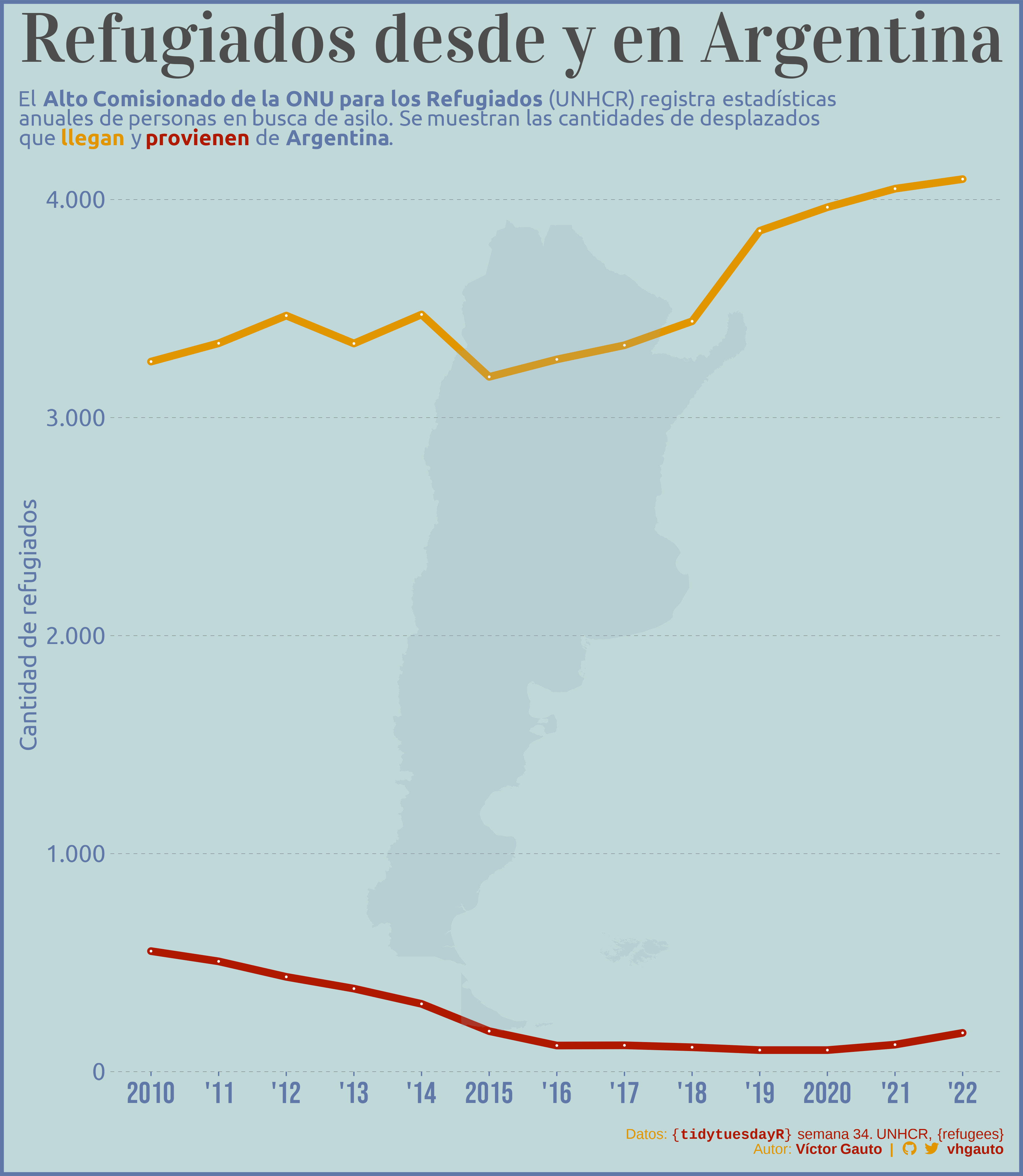
mi_title <- "Refugiados desde y en Argentina"

mi_subtitle <- glue(
  "El **Alto Comisionado de la ONU para los Refugiados** (UNHCR)
  registra estadísticas<br>
  anuales de personas en busca de asilo. 
  Se muestran las cantidades de desplazados<br>
  que <span style='color:{c2}'>**llegan**</span> y 
  <span style='color:{c3}'>**provienen**</span> de **Argentina**."
)

# figura de líneas, cantidad de refugiados ~ años
gg_ref <- arg |> 
  ggplot(aes(año, n, color = estado)) +
  geom_hline(
    yintercept = seq(0, 4000, 1000), color = c5, linewidth = .1, linetype = "ff") +
  geom_line(show.legend = FALSE, linewidth = 3, lineend = "round") +
  geom_point(show.legend = FALSE, color = "white", size = .4) +
  scale_x_continuous(breaks = 2010:2022, labels = eje_x_label) +
  scale_y_continuous(
    breaks = seq(0, 4000, 1000),
    labels = scales::label_number(big.mark = ".", decimal.mark = ","),
    expand = c(0, 0)) +
  scale_color_manual(values = c(c2, c3)) +
  coord_cartesian(clip = "off") +
  labs(
    x = NULL,
    y = "Cantidad de refugiados",
    title = mi_title,
    subtitle = mi_subtitle,
    caption = mi_caption) +
  theme_minimal() +
  theme(
    aspect.ratio = 1,
    plot.margin = margin(5.5, 11, 5.5, 11),
    plot.title.position = "plot",
    plot.title = element_text(size = 58, family = "vidaloka", color = c5),
    plot.subtitle = element_markdown(
      size = 18, color = c4, family = "ubuntu", margin = margin(5, 0, 25, 0)),
    plot.caption = element_markdown(
      color = c2, size = 12, margin = margin(20, 0, 5, 0)),
    axis.title.y = element_text(color = c4, family = "ubuntu", size = 20),
    axis.text.x = element_text(color = c4, family = "bebas", size = 25, margin = margin(5, 0, 0, 0)),
    axis.text.y = element_text(color = c4, family = "ubuntu", size = 20),
    axis.ticks.x = element_line(color = c4),
    axis.ticks.length.x = unit(.25, "line"),
    panel.grid = element_blank()
  )

# combino ambas figuras, con el mapa de Argentina de fondo
g <- gg_ref + 
  inset_element(
    gg_arg, left = .2, bottom = 0, right = .8, top = 1) +
  plot_annotation(
    theme = theme(
      plot.background = element_rect(fill = c1, color = c4, linewidth = 3)
    ))

# guardo
ggsave(
  plot = g,
  filename = "2023/semana_34/viz.png",
  width = 30,
  height = 34.5,
  units = "cm")

# abro
browseURL("2023/semana_34/viz.png")

Figura