Semana 15

Figura semana 15

Ciudades alcanzadas total o parcialmente por los eclipses solares de 2023 y 2024, en EE.UU.

Script

# paquetes ----------------------------------------------------------------

library(glue)
library(ggtext)
library(showtext)
library(sf)
library(tidyverse)

# fuente ------------------------------------------------------------------

# colores
c1 <- "#4B3232"
c2 <- "white"
c3 <- "gold"
c4 <- "black"

# fuente: Ubuntu
font_add(
  family = "ubuntu", 
  regular = "fuente/Ubuntu-Regular.ttf",
  bold = "fuente/Ubuntu-Bold.ttf",
  italic = "fuente/Ubuntu-Italic.ttf")

# fuente: Victor
font_add(
  family = "victor", 
  regular = "fuente/VictorMono-ExtraLight.ttf",
  bold = "fuente/VictorMono-VariableFont_wght.ttf",
  italic = "fuente/VictorMono-ExtraLightItalic.ttf")

# íconos
font_add(
  family = "jet", 
  regular = "fuente/JetBrainsMonoNLNerdFontMono-Regular.ttf")

showtext_auto()
showtext_opts(dpi = 300)

# caption
fuente <- glue(
  "Datos: <span style='color:{c3};'><span style='font-family:mono;'>",
  "{{<b>tidytuesdayR</b>}}</span> semana {15}. ",
  "Scientific Visualization Studio, <b>NASA</b>.</span>")
autor <- glue("<span style='color:{c3};'>**Víctor Gauto**</span>")
icon_twitter <- glue("<span style='font-family:jet;'>&#xf099;</span>")
icon_instagram <- glue("<span style='font-family:jet;'>&#xf16d;</span>")
icon_github <- glue("<span style='font-family:jet;'>&#xf09b;</span>")
icon_mastodon <- glue("<span style='font-family:jet;'>&#xf0ad1;</span>")
usuario <- glue("<span style='color:{c3};'>**vhgauto**</span>")
sep <- glue("**|**")

mi_caption <- glue(
  "{fuente}<br>{autor} {sep} {icon_github} {icon_twitter} {icon_instagram} ",
  "{icon_mastodon} {usuario}")

# datos -------------------------------------------------------------------

tuesdata <- tidytuesdayR::tt_load(2024, 15)

# me interesa distinguir las ciudades con eclipse total de las ciudades con 
# eclipse parcial, y agregar los horarios en rangos de 10min
ecl_2023 <- tuesdata$eclipse_annular_2023
par_2023 <- tuesdata$eclipse_partial_2023

ecl_2024 <- tuesdata$eclipse_total_2024
par_2024 <- tuesdata$eclipse_partial_2024

# EE.UU.
# quito estos estados
no_estados <- c(
  "Alaska", "Hawaii", "Commonwealth of the Northern Mariana Islands", "Guam", 
  "Puerto Rico", "United States Virgin Islands", "American Samoa")

# combino los estados y cambio de proyección
usa <- rgeoboundaries::gb_adm1(country = "USA") |> 
  filter(!shapeName %in% no_estados) |> 
  st_union() |> 
  st_transform(crs = 5070)

# función que convierte tibble en sf y calcula el tiempo (hora:minuto)
f_sf <- function(df, año, paleta = "tokyo") {
  d <- df |> 
    mutate(minuto = minute(eclipse_3), hora = hour(eclipse_3)) |> 
    mutate(minuto = minuto - minuto %% 10) |>
    select(lat, lon, hora, minuto) |> 
    mutate(hora_minuto = hm(glue("{hora}:{minuto}"))) |> 
    mutate(hm_fct = glue("{hora}:{minuto}")) |> 
    mutate(hm_fct = if_else(hm_fct == "19:0", "19:00", hm_fct)) |> 
    mutate(hm_fct = fct_reorder(hm_fct, hora_minuto)) |> 
    st_as_sf(coords = c("lon", "lat")) |> 
    st_set_crs(value = 4326) |> 
    st_transform(crs = 5070) |> 
    mutate(year = año)
  
  p <- scico::scico(n = length(unique(d$hm_fct)), palette = paleta)
  
  d |> 
    mutate(color = p[hm_fct])
}

# función que obtiene el centro de cada región hora:minuto
f_centro <- function(df, año) {
  df |> 
    select(hm_fct) |> 
    nest(.by = hm_fct) |> 
    mutate(uni = map(.x = data, ~ st_union(.x))) |> 
    mutate(centro = map(.x = uni, ~ st_centroid(.x))) |> 
    unnest(centro) |> 
    select(hm_fct, centro) |> 
    st_as_sf() |> 
    mutate(year = año) |> 
    mutate(coord = map(.x = centro, st_coordinates)) |> 
    mutate(coord = map(.x = coord, as_tibble)) |> 
    unnest(coord) |> 
    st_drop_geometry() |> 
    mutate(
      X = if_else(year == 2023, X + 1.6e5, X - 1.6e5),
      Y = if_else(year == 2023, Y + 1.1e5, Y + 1.2e5)) |> 
    mutate(angle = if_else(year == 2023, -45, 43)) |> 
    st_as_sf(coords = c("X", "Y")) |> 
    st_set_crs(value = 5070)
}

# función para convertir tibble a sf, para otras ciudades
f_parcial <- function(df, año) {
  df |> 
    st_as_sf(coords = c("lon", "lat")) |> 
    st_set_crs(value = 4326) |> 
    st_transform(crs = 5070) |> 
    mutate(year = año) |> 
    st_crop(usa) |> 
    select(year)
}

# ciudades con eclipse total
d_2023 <- f_sf(ecl_2023, 2023, paleta = "hawaii")
d_2024 <- f_sf(ecl_2024, 2024, paleta = "hawaii")

d <- rbind(d_2023, d_2024)

# horarios ubicados en el centro de las regiones
d_centro_2023 <- f_centro(d_2023, 2023)
d_centro_2024 <- f_centro(d_2024, 2024)

d_centro <- rbind(d_centro_2023, d_centro_2024) |> 
  mutate(coord = map(.x = geometry, st_coordinates)) |> 
  mutate(coord = map(.x = coord, as_tibble)) |> 
  unnest(coord) |> 
  st_drop_geometry()

# ciudades con eclipse parcial
d_parcial_2023 <- f_parcial(par_2023, 2023)
d_parcial_2024 <- f_parcial(par_2024, 2024)

d_parcial <- rbind(d_parcial_2023, d_parcial_2024)

# figura ------------------------------------------------------------------

# subtítulo
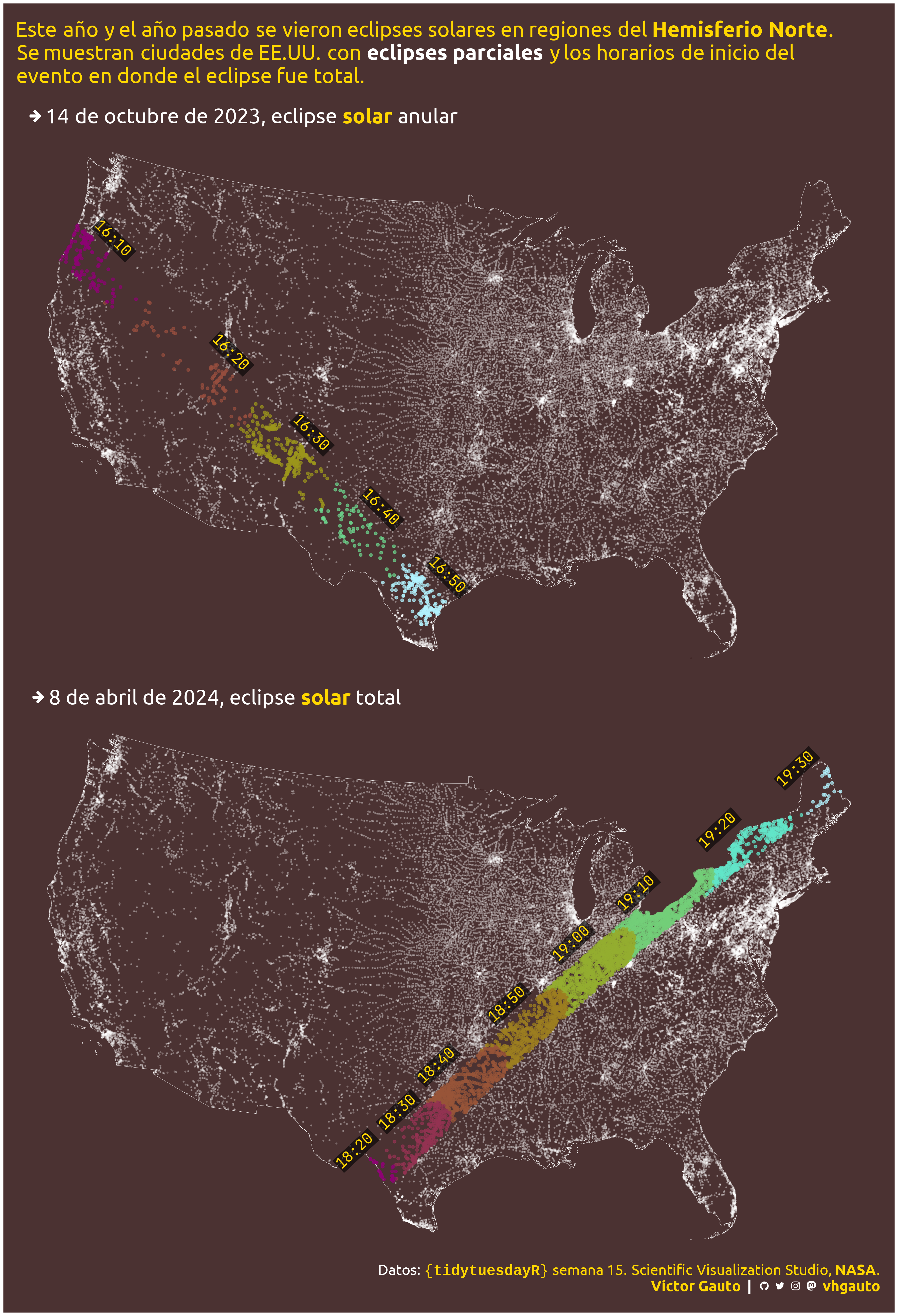
mi_subtitle <- glue(
  "Este año y el año pasado se vieron eclipses solares en regiones del ",
  "<b>Hemisferio Norte</b>.<br>",
  "Se muestran ciudades de EE.UU. con ",
  "<b style='color:{c2}'>eclipses parciales</b> y los horarios de inicio del<br>",
  "evento en donde el eclipse fue total."
)

# años de los eclipses
flecha_icon <- "<span style='font-family:jet;font-size:20pt;'>&#xf061;</span>"

label_año <- c(
  glue(
    "{flecha_icon} 14 de octubre de 2023, eclipse ",
    "<b style='color:gold'>solar</b> anular"), 
  glue(
    "{flecha_icon} 8 de abril de 2024, eclipse ",
    "<b style='color:gold'>solar</b> total"))
names(label_año) <- c(2023, 2024)

# figura
g <- ggplot() +
  # USA
  geom_sf(data = usa, fill = NA, color = c2, linewidth = .1) +
  # otras ciudades
  geom_sf(data = d_parcial, color = c2, size = .25, alpha = .25) +
  # eclipse
  geom_sf(
    data = d, aes(color = color), size = 1, alpha = .7, show.legend = FALSE) +
  # horas:minutos
  geom_richtext(
    data = d_centro, aes(X, Y, label = hm_fct, angle = angle), color = c3, 
    size = 5, hjust = .5, family = "jet", fill = alpha(c4, .6), 
    label.r = unit(0, "mm"), label.color = NA, 
    label.padding = unit(c(.1, .1, .1, .1), "lines")) +
  facet_wrap(vars(year), ncol = 1, labeller = as_labeller(label_año)) +
  # escalas
  scale_color_identity() +
  labs(subtitle = mi_subtitle, caption = mi_caption) +
  guides(
    color = guide_legend(override.aes = list(alpha = 1, size = 5, shape = 15))
  ) +
  theme_void() +
  theme(
    plot.background = element_rect(fill = c1, color = c2, linewidth = 3),
    plot.subtitle = element_markdown(
      family = "ubuntu", color = c3, size = 20, 
      margin = margin(b = 20, t = 10, l = 10), lineheight = unit(1.1, "line")),
    plot.margin = margin(t = 11, r = 6.4, b = 11, l = 6.4),
    plot.caption = element_markdown(
      color = c2, family = "ubuntu", size = 14, lineheight = unit(1.1, "line"),
      margin = margin(b = 10, r = 10)),
    strip.text = element_markdown(
      family = "ubuntu", color = c2, size = 20, hjust = .05)
  )

# guardo
ggsave(
  plot = g,
  filename = "2024/s15/viz.png",
  width = 30,
  height = 44,
  units = "cm")

# abro
browseURL("2024/s15/viz.png")

Figura