# paquetes ----------------------------------------------------------------
library(glue)
library(ggtext)
library(ggh4x)
library(showtext)
library(tidytext)
library(tidyverse)
# fuente ------------------------------------------------------------------
# colores
col <- MoMAColors::moma.colors(palette_name = "Smith")
# col <- MoMAColors::moma.colors(palette_name = "Budnitz")
c1 <- "grey40"
c2 <- "white"
# fuente: Ubuntu
font_add(
family = "ubuntu",
regular = "fuente/Ubuntu-Regular.ttf",
bold = "fuente/Ubuntu-Bold.ttf",
italic = "fuente/Ubuntu-Italic.ttf"
)
# monoespacio & íconos
font_add(
family = "jet",
regular = "fuente/JetBrainsMonoNLNerdFontMono-Regular.ttf"
)
showtext_auto()
showtext_opts(dpi = 300)
# caption
fuente <- glue(
"Datos: <span style='color:{col[4]};'><span style='font-family:jet;'>",
"{{<b>tidytuesdayR</b>}}</span> semana {43}, ",
"<b>CIA World Factbook</b>.</span>"
)
autor <- glue("<span style='color:{col[4]};'>**Víctor Gauto**</span>")
icon_twitter <- glue("<span style='font-family:jet;'></span>")
icon_instagram <- glue("<span style='font-family:jet;'></span>")
icon_github <- glue("<span style='font-family:jet;'></span>")
icon_mastodon <- glue("<span style='font-family:jet;'>󰫑</span>")
usuario <- glue("<span style='color:{col[4]};'>**vhgauto**</span>")
sep <- glue("**|**")
mi_caption <- glue(
"{fuente}<br>{autor} {sep} {icon_github} {icon_twitter} {icon_instagram} ",
"{icon_mastodon} {usuario}"
)
# datos -------------------------------------------------------------------
tuesdata <- tidytuesdayR::tt_load(2024, 43)
cia <- tuesdata$cia_factbook
# me interesa la posición de Argentina respecto del resto de los países
# parámetros de interés y sus traducciones
param_c <- c("area", "life_exp_at_birth", "population", "internet_ratio")
param_trad <- c(
glue("<b style='color: {col[1]}'>Superficie (km<sup>2</sup>)</b>"),
glue("<b style='color: {col[2]}'>Expectativa de vida</b>"),
glue("<b style='color: {col[3]}'>Población</b>"),
glue("<b style='color: {col[4]}'>Población que usa internet (%)</b>")
)
names(param_trad) <- param_c
# acomodo los datos y obtengo el porcentaje de personas con internet
d <- cia |>
select(country, area, internet_users, life_exp_at_birth, population) |>
mutate(
internet_ratio = internet_users/population*100
) |>
drop_na() |>
pivot_longer(
cols = -country,
names_to = "param",
values_to = "valor"
) |>
mutate(
arg = if_else(
country == "Argentina",
"Arg",
param
)
) |>
filter(param != "internet_users") |>
mutate(trad = param_trad[param])
# figura ------------------------------------------------------------------
# cantidad de países y grilla de posiciones
n_pais <- length(unique(d$country))
grid_label <- tibble(
x = 1:n_pais,
y = Inf,
label = rev(x)
) |>
filter(label == label - (label %% 25) | x == n_pais) |>
mutate(label = glue("#{label}"))
# escalas individuales del eje vertical (facetas)
ejes_y <- list(
# espectativa de vida
scale_y_continuous(
breaks = seq(0, 100, 20),
limits = c(0, 100),
expand = c(0, 0)
),
# población
scale_y_log10(
breaks = 10^(0:9),
limits = c(1, 10^9),
labels = format(
10^(0:9), scientific = FALSE, big.mark = ".", decimal.mark = ","
)
),
# internet
scale_y_continuous(
breaks = seq(0, 100, 20),
limits = c(0, 100),
expand = c(0, 0)
),
# superficie
scale_y_log10(
breaks = 10^(0:9),
labels = format(
10^(0:9), scientific = FALSE, big.mark = ".", decimal.mark = ","
)
)
)
# bandera e ícono
bandera <- glue(
"https://upload.wikimedia.org/wikipedia/commons/thumb/1/1a/",
"Flag_of_Argentina.svg/320px-Flag_of_Argentina.svg.png"
)
triangulo <- glue("<span style='font-family:jet;'>󱨉</span>")
# posición de Argentina en cada parámetro
d_arg <- d |>
arrange(param, desc(valor)) |>
mutate(pos = row_number(), .by = param) |>
filter(country == "Argentina") |>
mutate(
label = glue(
"#{pos}<br><img src='{bandera}' width=30></img><br>{triangulo}"
)
)
# parámetros y estilo de c/u para el subtítulo
p1 <- glue("<b style='color: {col[2]};'>expectativa de vida</b>")
p2 <- glue("<b style='color: {col[3]};'>población</b>")
p3 <- glue("<b style='color: {col[4]};'>acceso a internet</b>")
p4 <- glue("<b style='color: {col[1]};'>superficie</b>")
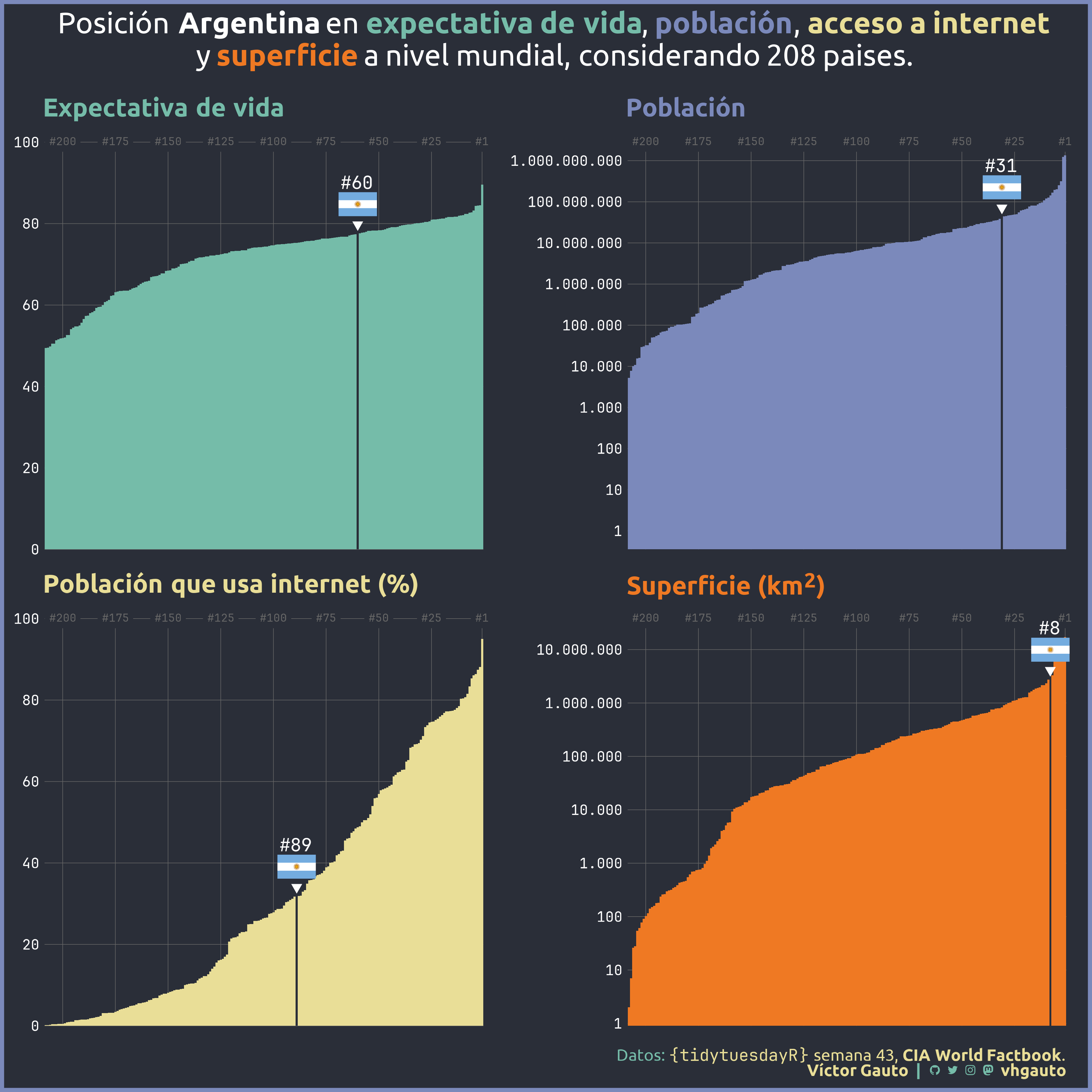
mi_subtítulo <- glue(
"Posición <b>Argentina</b> en {p1}, {p2}, {p3}<br>y {p4} a nivel mundial, ",
"considerando 208 paises."
)
# figura
g <- ggplot(d, aes(reorder_within(country, valor, trad), valor, fill = arg)) +
geom_vline(
data = grid_label, aes(xintercept = x), color = c1, linewidth = .2
) +
geom_col(color = NA, show.legend = FALSE, width = 1) +
geom_richtext(
data = grid_label, aes(x, y, label = label), inherit.aes = FALSE,
family = "jet", label.color = NA, fill = col[5], color = c1, size = 3
) +
geom_richtext(
data = d_arg, aes(label = label), fill = NA, label.color = NA, vjust = .1,
size = 5, color = c2, lineheight = .1, family = "jet"
) +
facet_wrap(vars(trad), ncol = 2, scales = "free") +
coord_cartesian(clip = "off") +
facetted_pos_scales(y = ejes_y) +
scale_fill_manual(
breaks = unique(d$arg),
values = as.character(c(col))
) +
labs(x = NULL, y = NULL, subtitle = mi_subtítulo, caption = mi_caption) +
theme_classic() +
theme(
plot.margin = margin(r = 20, l = 10),
plot.background = element_rect(
fill = col[5], color = col[3], linewidth = 3
),
plot.subtitle = element_markdown(
family = "ubuntu", size = 23, hjust = .5, color = c2,
lineheight = unit(1.1, "line"), margin = margin(b = 20, t = 10)
),
plot.caption = element_markdown(
family = "ubuntu", size = 13, color = col[2],
margin = margin(b = 10, t = 15)
),
axis.ticks = element_blank(),
axis.text = element_text(family = "jet", color = c2, size = 11),
axis.text.x = element_blank(),
axis.line = element_blank(),
panel.background = element_rect(fill = col[5]),
panel.grid.major.y = element_line(color = c1, linewidth = .2),
panel.grid.major.x = element_blank(),
panel.grid.minor.x = element_blank(),
panel.spacing.x = unit(1.5, "line"),
panel.spacing.y = unit(1.1, "line"),
panel.border = element_blank(),
strip.background = element_blank(),
strip.text = element_markdown(
family = "ubuntu", hjust = 0, size = 20, color = col[4],
margin = margin(b = 15)
)
)
# guardo
ggsave(
plot = g,
filename = "2024/s43/viz.png",
width = 30,
height = 30,
units = "cm"
)
# abro
browseURL(glue("{getwd()}/2024/s43/viz.png"))