Ocultar código
library(glue)
library(ggtext)
library(showtext)
library(patchwork)
library(terra)
library(magick)
library(tidyterra)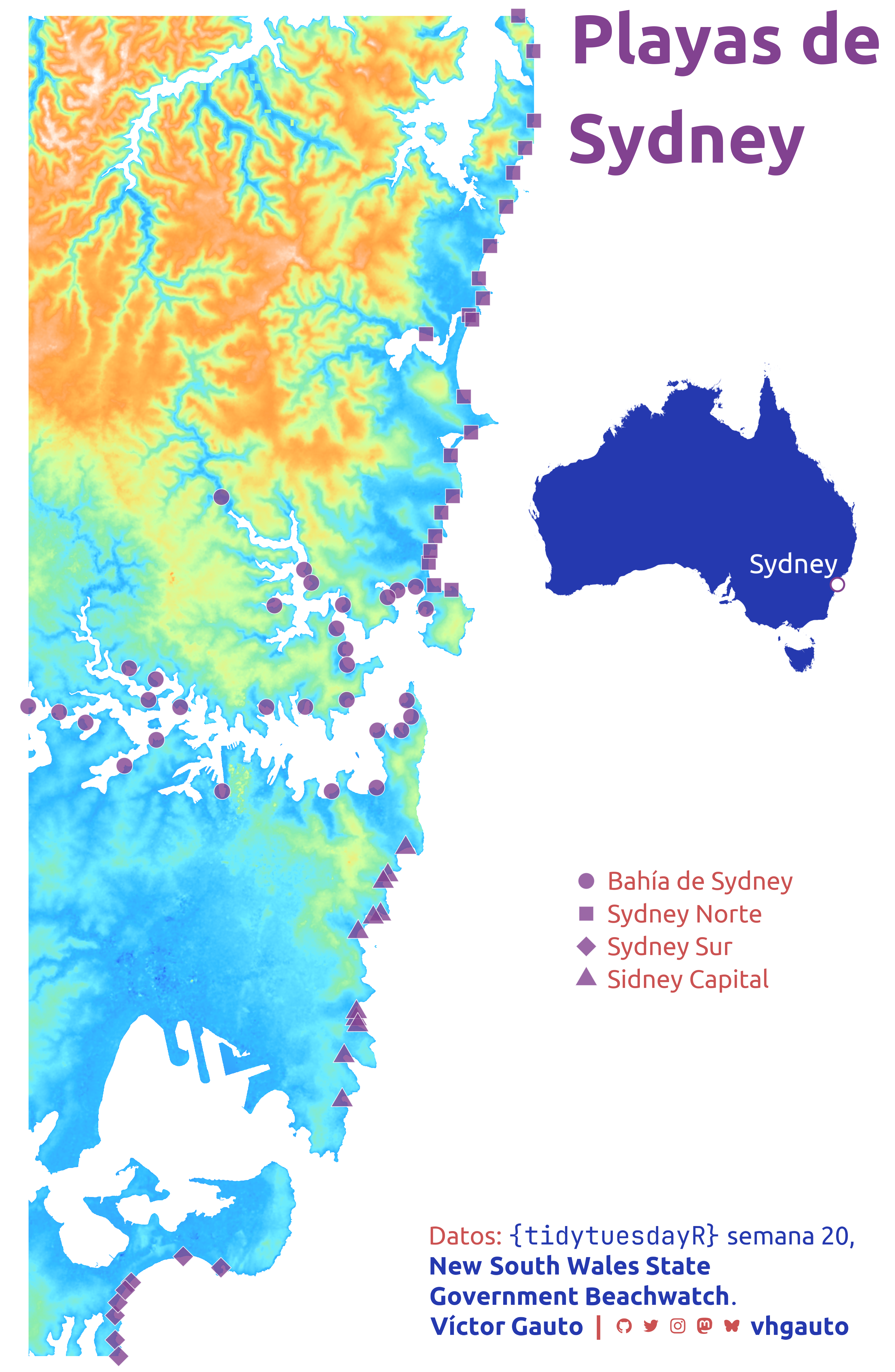
library(tidyverse)Playas en Sydney, Australia, indicando la región a la que pertenecen.
library(glue)
library(ggtext)
library(showtext)
library(patchwork)
library(terra)
library(magick)
library(tidyterra)
library(tidyverse)Colores.
c1 <- "#2539AF"
c2 <- "#CB5252"
c3 <- "#824290"
c4 <- "white"
Fuentes: Ubuntu y JetBrains Mono.
font_add(
  family = "ubuntu",
  regular = "././fuente/Ubuntu-Regular.ttf",
  bold = "././fuente/Ubuntu-Bold.ttf",
  italic = "././fuente/Ubuntu-Italic.ttf"
)

font_add(
  family = "jet",
  regular = "././fuente/JetBrainsMonoNLNerdFontMono-Regular.ttf"
)

showtext_auto()
showtext_opts(dpi = 300)fuente <- glue(
"Datos: <span style='color:{c1};'><span style='font-family:jet;'>",
"{{<b>tidytuesdayR</b>}}</span> semana 20,<br>",
"<b>New South Wales State<br>Government Beachwatch</b>.</span>"
)
autor <- glue("<span style='color:{c1};'>**Víctor Gauto**</span>")
icon_twitter <- glue("<span style='font-family:jet;'></span>")
icon_instagram <- glue("<span style='font-family:jet;'></span>")
icon_github <- glue("<span style='font-family:jet;'></span>")
icon_mastodon <- glue("<span style='font-family:jet;'>󰫑</span>")
icon_bsky <- glue("<span style='font-family:jet;'></span>")
usuario <- glue("<span style='color:{c1};'>**vhgauto**</span>")
sep <- glue("**|**")
mi_caption <- glue(
"{fuente}<br>{autor} {sep} {icon_github} {icon_twitter} {icon_instagram} ",
"{icon_mastodon} {icon_bsky} {usuario}"
)tuesdata <- tidytuesdayR::tt_load(2025, 20)
water_quality <- tuesdata$water_qualityMe interesa la posición de las playas y la región.
Remuevo playas que se encuentran en el extremo Oeste, removiendo aquellas playas que tengan valores mínimos de longitud geográfica.
lon <- water_quality |>
  distinct(longitude) %>%
  slice_max(order_by = longitude, n = nrow(.)-7)
Al combinar las longitudes geográficas con los datos, convierto a vector y obtengo su extensión.
v <- water_quality |>
  select(region, latitude, longitude) |>
  inner_join(lon, by = join_by(longitude)) |>
  distinct() |>
  vect(geom = c("longitude", "latitude"), crs = "EPSG:4326")

bbox <- vect(ext(v), crs(v))
Obtengo el vector de Australia, recorto a la región de las playas y descargo el ráster de elevación.
aus <- rgeoboundaries::gb_adm0(country = "AUS") |>
  vect()

aus_crop <- terra::crop(aus, bbox)

elev_r <- elevatr::get_elev_raster(
  locations = sf::st_as_sf(aus_crop),
  z = 13,
  clip = "locations"
) |>
  rast()
Remuevo valores anormales con una mediana de ventana 3x3 y renombro la variable.
elev <- terra::focal(elev_r, w = 3, fun = median)
names(elev) <- "altura"
elev[elev < -50] <- NA
Recorto el vector de Australia.
bbox_aus <- ext(110, 157, ext(aus)$ymin, ext(aus)$ymax) |>
  vect(crs = crs(aus))

aus_mapa <- crop(aus, bbox_aus)El mapa final está compuesto de dos figuras: el mapa principal de las playas en Sydney, y uno más pequeño con el mapa de Australia, indicando la región de interés.
Vector punto de la ciudad de Sydney.
sydney <- tibble(
  x = 151.2,
  y = -33.866667,
  label = "Sydney"
) |>
  vect(geom = c("x", "y"), crs = crs(v))
Creo mapa indicando la ubicación y nombre de Sydney. Guardo figura.
g_aus <- ggplot() +
  geom_spatvector(data = aus_mapa, fill = c1, color = NA) +
  geom_spatvector(
    data = sydney, size = 4, color = c3, shape = 21, fill = c4, stroke = 1
  ) +
  geom_spatvector_text(
    data = sydney, aes(label = label), hjust = 1, vjust = -.6, color = c4,
    family = "ubuntu", size = 7
  ) +
  coord_sf(expand = FALSE) +
  theme_void() +
  theme(
    plot.margin = margin(0, 0, 0, 0),
    plot.background = element_blank()
  )

ggsave(
  plot = g_aus,
  filename = "tidytuesday/2025/australia.png",
  width = 1000,
  height = 1000,
  units = "px"
)Creo una función para indicar la posición vertical de las anotaciones según la fracción de la altura disponible.
altura_label <- function(x) ext(bbox)$ymin + (ext(bbox)$ymax-ext(bbox)$ymin)*xCreo subtítulo, fuente de datos y autor.
mi_subitulo_tbl <- tibble(
  x = ext(bbox)$xmax*1.0001,
  y = altura_label(1),
  label = "Playas de\nSydney"
) |>
  vect(geom = c("x", "y"), crs = crs(v))

mi_caption_tbl <- tibble(
  x = ext(bbox)$xmax*.9997,
  y = altura_label(.1),
  label = mi_caption
)
Mapa con la ubicación de las playas. Guardo la figura.
g <- ggplot() +
  geom_spatraster(
    data = elev, aes(fill = altura),
    maxcell = prod(dim(elev)),
    show.legend = FALSE
  ) +
  geom_spatvector(
    data = v, aes(shape = region), size = 7, alpha = .8, fill = c3,
    color = c4
  ) +
  geom_spatvector_text(
    data = mi_subitulo_tbl, aes(label = label), family = "ubuntu", size = 23,
    hjust = 0, vjust = 1, color = c3, fontface = "bold"
  ) +
  geom_richtext(
    data = mi_caption_tbl, aes(x, y, label = label), inherit.aes = FALSE,
    size = 24/.pt, hjust = 0, vjust = 1, family = "ubuntu", fill = NA,
    label.colour = NA, color = c2
  ) +
  scale_fill_grass_c(palette = "haxby") +
  scale_shape_manual(
    breaks = unique(v$region),
    values = c(21, 22, 23, 24),
    labels = c(
      "Bahía de Sydney", "Sydney Norte", "Sydney Sur", "Sidney Capital"
    )
  ) +
  coord_sf(expand = FALSE, clip = "off") +
  labs(shape = NULL) +
  theme_void(base_family = "ubuntu", base_size = 20) +
  theme(
    plot.margin = margin(r = 80, t = 15, l = 10, b = 15),
    plot.background = element_rect(fill = c4, color = NA),
    legend.position = "right",
    legend.justification.right = c(.5, .3),
    legend.text = element_text(size = rel(1.2), color = c2),
    legend.key.spacing.y = unit(10, "pt")
  )

ggsave(
  plot = g,
  filename = "tidytuesday/2025/playa.png",
  width = 30,
  height = 46,
  units = "cm"
)Leo ambos mapas y agrego el de Australia, de menor tamaño, sobre el mapa de playas. Guardo la figura final.
img_aus <- image_read("tidytuesday/2025/australia.png") |>
  image_scale(geometry = "1300x")

img_playa <- image_read("tidytuesday/2025/playa.png")

img_playa |>
  image_composite(img_aus, gravity = "northeast", offset = "+150+1400") |>
  image_write(path = "tidytuesday/2025/semana_20.png")