Semana 48

Figura semana 48

Encuentros en las fronteras Norte y Sur de Estados Unidos.

Script

#
# paquetes ----------------------------------------------------------------

library(glue)
library(ggtext)
library(showtext)
library(ggbump)
library(tidyverse)

# fuente ------------------------------------------------------------------

# colores
cc <- c("#451B40", "#324D5A", "#589445", "#B5003C")
c1 <- "grey70"
c2 <- "grey95"
c3 <- "black"

# fuente: Ubuntu
font_add(
  family = "ubuntu",
  regular = "fuente/Ubuntu-Regular.ttf",
  bold = "fuente/Ubuntu-Bold.ttf",
  italic = "fuente/Ubuntu-Italic.ttf"
)

# monoespacio & íconos
font_add(
  family = "jet",
  regular = "fuente/JetBrainsMonoNLNerdFontMono-Regular.ttf"
)

# bebas neue
font_add(
  family = "bebas",
  regular = "fuente/BebasNeue-Regular.ttf"
)

showtext_auto()
showtext_opts(dpi = 300)

# caption
fuente <- glue(
  "Datos: <span style='color:{cc[1]};'><span style='font-family:jet;'>",
  "{{<b>tidytuesdayR</b>}}</span> semana {48}, ",
  "<b>U.S. Customs and Border Protection</b>.</span>"
)
autor <- glue("<span style='color:{cc[1]};'>**Víctor Gauto**</span>")
icon_twitter <- glue("<span style='font-family:jet;'>&#xf099;</span>")
icon_instagram <- glue("<span style='font-family:jet;'>&#xf16d;</span>")
icon_github <- glue("<span style='font-family:jet;'>&#xf09b;</span>")
icon_mastodon <- glue("<span style='font-family:jet;'>&#xf0ad1;</span>")
icon_bsky <- glue("<span style='font-family:jet;'>&#xe28e;</span>")
usuario <- glue("<span style='color:{cc[1]};'>**vhgauto**</span>")
sep <- glue("**|**")

mi_caption <- glue(
  "{fuente}<br>{autor} {sep} {icon_github} {icon_twitter} {icon_instagram} ",
  "{icon_mastodon} {icon_bsky} {usuario}"
)

# datos -------------------------------------------------------------------

tuesdata <- tidytuesdayR::tt_load(2024, 48)
cbp_resp <- tuesdata$cbp_resp

# me interesan los países más frecuentes y su evolución anual

top_paises <- 20

# función para generar los datos por frontera N/S

f_frontera <- function(frontera, frontera_label) {
  cbp_resp |>
    filter(land_border_region == frontera) |>
    select(fiscal_year, citizenship) |>
    count(citizenship, fiscal_year) |>
    filter(citizenship != "OTHER") |>
    slice_max(order_by = n, by = fiscal_year, n = top_paises) |>
    arrange(fiscal_year, desc(n)) |>
    mutate(puesto = row_number(), .by = fiscal_year) |>
    mutate(lado = frontera_label)
}

# combino datos frontera N/S
cbp_n <- f_frontera("Northern Land Border", "NORTE")
cbp_s <- f_frontera("Southwest Land Border", "SUR")

d <- rbind(cbp_n, cbp_s) |>
  mutate(citizenship = if_else(
    citizenship == "CHINA, PEOPLES REPUBLIC OF",
    "CHINA",
    citizenship
  ))

# agrego colores a las líneas y nombres de países
paises <- unique(d$citizenship)
colores <- rep(cc, 5)
names(colores) <- paises

d <- mutate(d, color = colores[citizenship]) |>
  mutate(
    puesto_label = if_else(puesto < 10, glue("0{puesto}"), glue("{puesto}"))
  )

# etiquetas de puestos, en años extremos
cbp_ext <- filter(d, fiscal_year == 2020 | fiscal_year == 2024) |>
  mutate(hjust = if_else(fiscal_year == 2020, 1, 0)) |>
  mutate(citizenship = str_to_title(citizenship))

# figura ------------------------------------------------------------------

# N/S y subtítulo
lugares <- tibble(
  fiscal_year = 2022,
  puesto = 3,
  lado = c("NORTE", "SUR"),
  color = c1
)

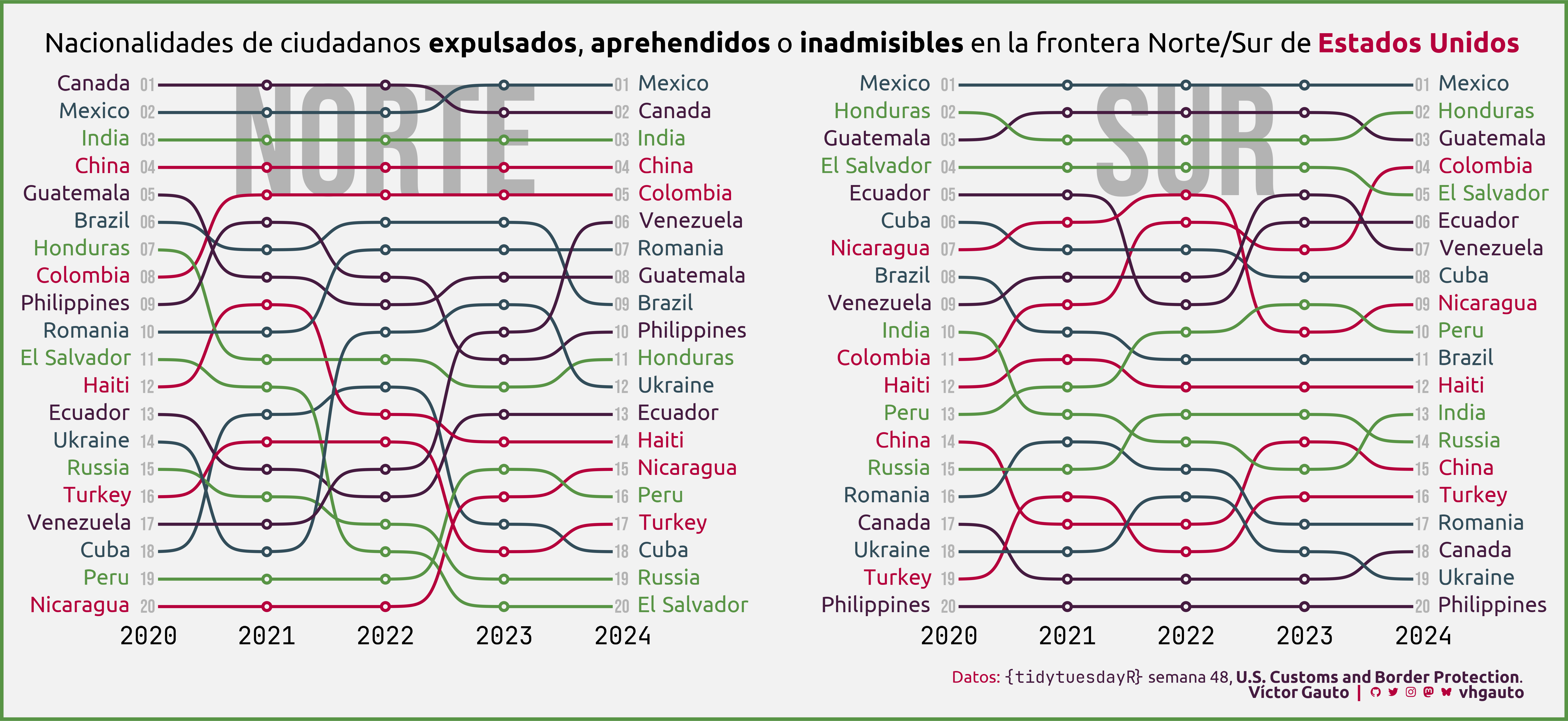
mi_subtitulo <- glue(
  "Nacionalidades de ciudadanos **expulsados**, **aprehendidos** o
  **inadmisibles** en la frontera Norte/Sur de
  <b style='color:{cc[4]}'>Estados Unidos</b>"
)

# figura
g <- ggplot(d, aes(fiscal_year, puesto, color = color, fill = color)) +
  # N & S
  geom_text(data = lugares, aes(label = lado), size = 50, family = "bebas") +
  # bump & puntos
  geom_bump(aes(group = citizenship), linewidth = 1.3, show.legend = FALSE) +
  geom_point(
    shape = 21, fill = c2, size = 2, stroke = 2, show.legend = FALSE
  ) +
  # izquierda
  geom_richtext(
    data = filter(cbp_ext, fiscal_year == 2020),
    aes(label = citizenship, hjust = hjust), fill = NA,
    size = 7, show.legend = FALSE, family = "ubuntu", label.color = NA,
    label.padding = unit(c(0, 15, 0, 0), "pt")
  ) +
  # derecha
  geom_richtext(
    data = filter(cbp_ext, fiscal_year == 2024),
    aes(label = citizenship, hjust = hjust), fill = NA,
    size = 7, show.legend = FALSE, family = "ubuntu", label.color = NA,
    label.padding = unit(c(0, 0, 0, 15), "pt")
  ) +
  # puestos
  geom_richtext(
    data = cbp_ext, aes(label = puesto_label), family = "bebas", size = 6,
    label.color = NA, color = c1, fill = c2, label.r = unit(5, "pt"),
    label.padding = unit(c(2, 2, 2, 2), "pt")
  ) +
  facet_wrap(vars(lado), ncol = 2, scales = "free") +
  scale_y_reverse(
    expand = c(0, 0)
  ) +
  scale_color_identity() +
  scale_fill_identity() +
  coord_cartesian(clip = "off") +
  labs(x = NULL, y = NULL, subtitle = mi_subtitulo, caption = mi_caption) +
  theme_minimal(base_size = 12) +
  theme(
    aspect.ratio = 1,
    plot.margin = margin(r = 110, l = 110, t = 30, b = 18),
    plot.background = element_rect(fill = c2, color = cc[3], linewidth = 3),
    plot.title.position = "plot",
    plot.subtitle = element_markdown(
      family = "ubuntu", color = c3, size = 25, margin = margin(b = 25),
      hjust = .5
    ),
    plot.caption = element_markdown(
      family = "ubuntu", color = cc[4], size = 15,
      margin = margin(t = 20, r = -70)
    ),
    panel.grid = element_blank(),
    panel.spacing.x = unit(250, "pt"),
    axis.text.x = element_text(
      family = "jet", size = 22, color = c3, margin = margin(t = 15)
    ),
    axis.text.y = element_blank(),
    strip.text = element_blank()
  )

# guardo
ggsave(
  plot = g,
  filename = "2024/s48/viz.png",
  width = 50,
  height = 23,
  units = "cm"
)

# abro
browseURL(glue("{getwd()}/2024/s48/viz.png"))

Figura