Ocultar código
library(glue)
library(ggtext)
library(showtext)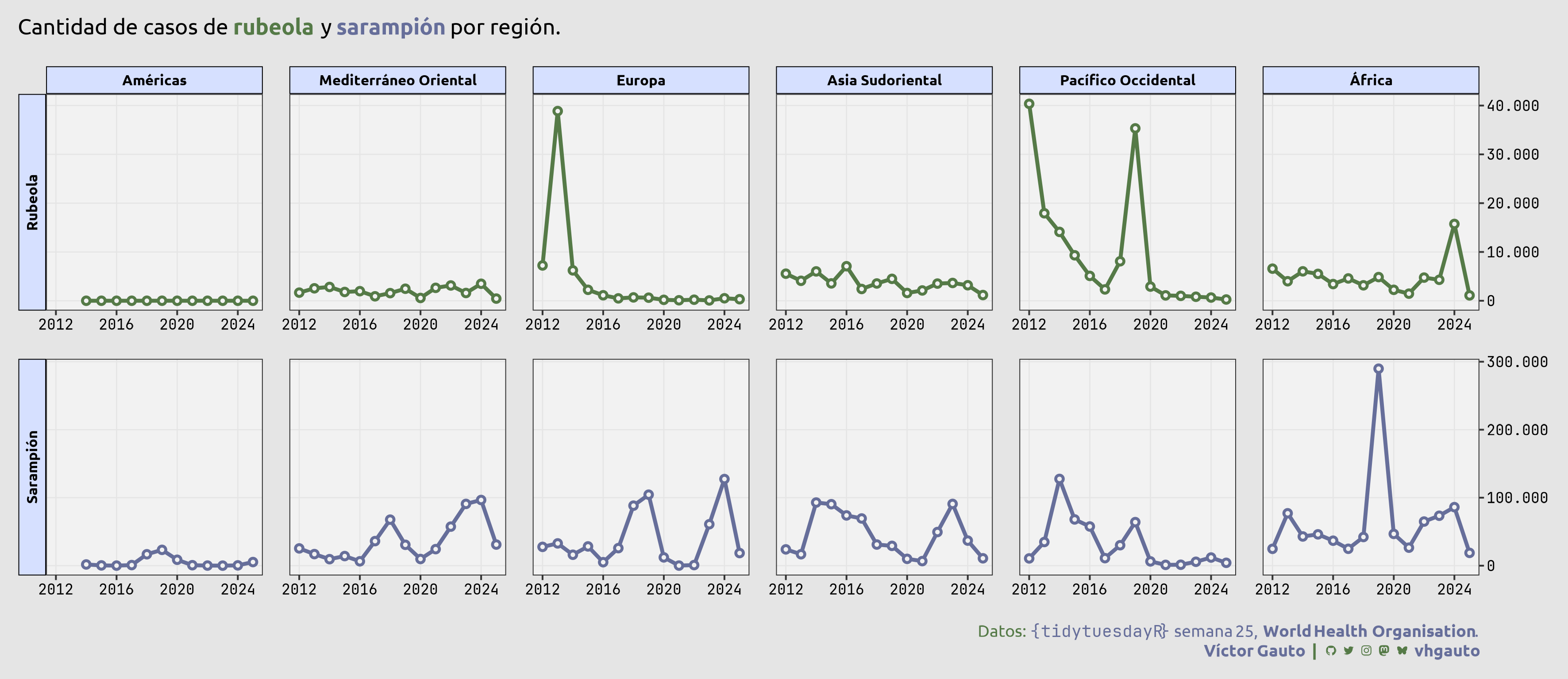
library(tidyverse)Cantidad de casos de rubeola y sarampión por región.
library(glue)
library(ggtext)
library(showtext)
library(tidyverse)Colores.
c1 <- "#666E9A"
c2 <- "#557A47"
c3 <- "#D6E0FF"
c4 <- "black"
c5 <- "grey90"
c6 <- "grey95"
Fuentes: Ubuntu y JetBrains Mono.
font_add(
  family = "ubuntu",
  regular = "././fuente/Ubuntu-Regular.ttf",
  bold = "././fuente/Ubuntu-Bold.ttf",
  italic = "././fuente/Ubuntu-Italic.ttf"
)

font_add(
  family = "jet",
  regular = "././fuente/JetBrainsMonoNLNerdFontMono-Regular.ttf"
)

showtext_auto()
showtext_opts(dpi = 300)fuente <- glue(
"Datos: <span style='color:{c1};'><span style='font-family:jet;'>",
"{{<b>tidytuesdayR</b>}}</span> semana 25, ",
"<b>World Health Organisation</b>.</span>"
)
autor <- glue("<span style='color:{c1};'>**Víctor Gauto**</span>")
icon_twitter <- glue("<span style='font-family:jet;'></span>")
icon_instagram <- glue("<span style='font-family:jet;'></span>")
icon_github <- glue("<span style='font-family:jet;'></span>")
icon_mastodon <- glue("<span style='font-family:jet;'>󰫑</span>")
icon_bsky <- glue("<span style='font-family:jet;'></span>")
usuario <- glue("<span style='color:{c1};'>**vhgauto**</span>")
sep <- glue("**|**")
mi_caption <- glue(
"{fuente}<br>{autor} {sep} {icon_github} {icon_twitter} {icon_instagram} ",
"{icon_mastodon} {icon_bsky} {usuario}"
)tuesdata <- tidytuesdayR::tt_load(2025, 25)
cases_month <- tuesdata$cases_month
cases_year <- tuesdata$cases_yearMe interesa la cantidad de casos por región, anualmente.
Sumo la cantidad anual, reordeno y agrego traducción a las regiones.
region_etq <- c(
  AFRO = "África",
  AMRO = "Américas",
  EMRO = "Mediterráneo Oriental",
  EURO = "Europa",
  SEARO = "Asia Sudoriental",
  WPRO = "Pacífico Occidental"
)

d <- cases_year |>
  reframe(
    Sarampión = sum(measles_total),
    Rubeola = sum(rubella_total),
    .by = c(region, year)
  ) |>
  pivot_longer(
    cols = c(Sarampión, Rubeola),
    names_to = "caso",
    values_to = "cantidad"
  ) |>
  mutate(reg = region_etq[region]) |>
  mutate(reg = fct_reorder(reg, cantidad)) |>
  mutate(
    caso = if_else(
      caso == "Sarampión",
      glue("<b style='color:{c1}'>Sarampión</b>"),
      glue("<b style='color:{c2}'>Rubeola</b>")
    )
)Título y figura.
mi_titulo <- glue(
  "Cantidad de casos de <b style='color: {c2}'>rubeola</b> y
  <b style='color: {c1}'>sarampión</b> por región."
)

g <- ggplot(d, aes(year, cantidad, color = caso)) +
  geom_line(linewidth = 1, show.legend = FALSE) +
  geom_point(size = 2, show.legend = FALSE) +
  geom_point(size = .5, color = c6, show.legend = FALSE) +
  facet_grid(caso ~ reg, scales = "free_y", switch = "y", axes = "all_x") +
  scale_x_continuous(breaks = scales::breaks_width(4)) +
  scale_y_continuous(
    position = "right",
    labels = scales::label_number(big.mark = ".", decimal.mark = ",")
  ) +
  scale_color_manual(
    values = c(c2, c1)
  ) +
  labs(x = NULL, y = NULL, title = mi_titulo, caption = mi_caption) +
  theme_bw(base_size = 10, base_family = "ubuntu") +
  theme(
    text = element_text(color = c4),
    plot.margin = margin(r = 10, l = 10),
    plot.background = element_rect(fill = c5, color = NA),
    plot.title = element_markdown(color = c4, margin = margin(b = 15)),
    plot.title.position = "plot",
    plot.caption = element_markdown(
      color = c2, size = rel(.9), margin = margin(t = 15), lineheight = 1.2
    ),
    aspect.ratio = 1,
    axis.text = element_text(family = "jet", color = c4),
    panel.background = element_rect(fill = c6),
    panel.grid.minor = element_blank(),
    panel.grid.major = element_line(color = c5, linewidth = .3),
    panel.spacing = unit(1, "line"),
    strip.background = element_rect(fill = c3, color = c4),
    strip.background.y = element_blank(),
    strip.text = element_markdown(face = "bold", color = c4),
    strip.text.y = element_markdown(size = rel(1.6))
  )
Guardo.
ggsave(
  plot = g,
  filename = "tidytuesday/2025/semana_25.png",
  width = 30,
  height = 13,
  units = "cm"
)