Ocultar código
library(glue)
library(ggtext)
library(showtext)
library(terra)
library(ggspatial)
library(tidyterra)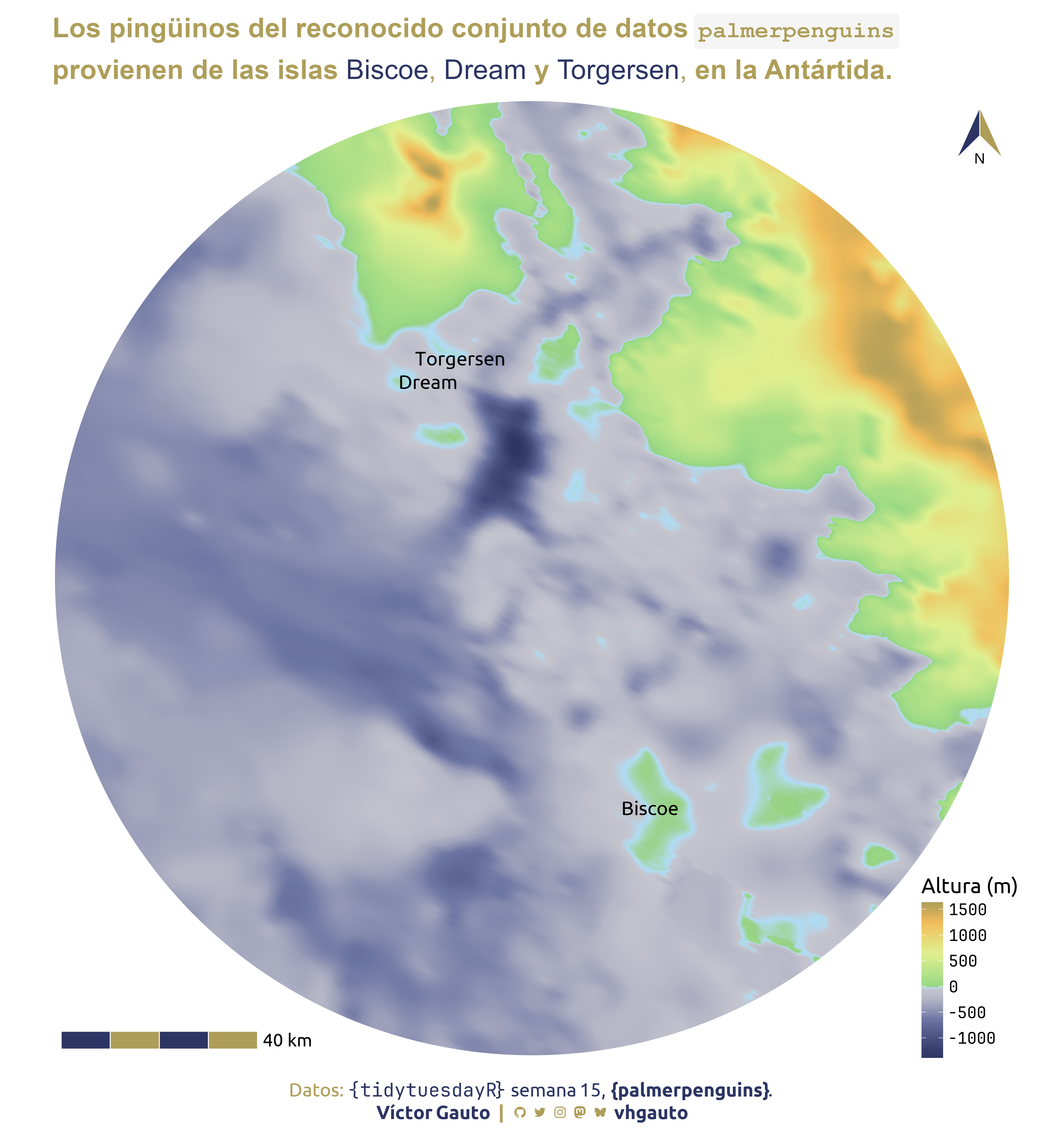
library(tidyverse)Mapa de elevación de las islas de pingüinos del paquete palmerpenguins.
library(glue)
library(ggtext)
library(showtext)
library(terra)
library(ggspatial)
library(tidyterra)
library(tidyverse)Colores.
c1 <- "#2C3563"
c2 <- "#AE9E59"
c3 <- "#AEDF87"
c4 <- "white"
Fuentes: Ubuntu y JetBrains Mono.
font_add(
  family = "ubuntu",
  regular = "././fuente/Ubuntu-Regular.ttf",
  bold = "././fuente/Ubuntu-Bold.ttf",
  italic = "././fuente/Ubuntu-Italic.ttf"
)

font_add(
  family = "jet",
  regular = "././fuente/JetBrainsMonoNLNerdFontMono-Regular.ttf"
)

showtext_auto()
showtext_opts(dpi = 300)fuente <- glue(
"Datos: <span style='color:{c1};'><span style='font-family:jet;'>",
"{{<b>tidytuesdayR</b>}}</span> semana 15, ",
"<b>{{palmerpenguins}}</b>.</span>"
)
autor <- glue("<span style='color:{c1};'>**Víctor Gauto**</span>")
icon_twitter <- glue("<span style='font-family:jet;'></span>")
icon_instagram <- glue("<span style='font-family:jet;'></span>")
icon_github <- glue("<span style='font-family:jet;'></span>")
icon_mastodon <- glue("<span style='font-family:jet;'>󰫑</span>")
icon_bsky <- glue("<span style='font-family:jet;'></span>")
usuario <- glue("<span style='color:{c1};'>**vhgauto**</span>")
sep <- glue("**|**")
mi_caption <- glue(
"{fuente}<br>{autor} {sep} {icon_github} {icon_twitter} {icon_instagram} ",
"{icon_mastodon} {icon_bsky} {usuario}"
)tuesdata <- tidytuesdayR::tt_load(2025, 15)Me interesa crear un mapa con las islas de los pingüinos.
Obtengo de Wikipedia las coordenadas de las islas Biscoe, Dream y Torgersen. Convierto a vector de puntos.
p <- tribble(
  ~x, ~y, ~isla,
  -65.5, -65.433333, "Biscoe",
  -64.233333, -64.733333, "Dream",
  -64.083333, -64.766667, "Torgersen"
) |>
  vect(geom = c("x", "y"), crs = "EPSG:4326") |>
  project("EPSG:3031")
Calculo el centroide de las tres islas y creo una circunferencia alrededor. Luego, descargo un modelo de elevación de la región de interés. Guardo el ráster descargado.
cent <- as.lines(p) |>
  centroids()

buf <- buffer(cent, 100000, quadsegs = 500)

r <- elevatr::get_elev_raster(
  locations = sf::st_as_sf(buf),
  z = 10,
  clip = "locations"
) |>
  rast()

writeRaster(r, "tidytuesday/2025/semana_15.tif", overwrite = TRUE)

r <- rast("tidytuesday/2025/semana_15.tif")Defino el estilo de la fecha que señala el Norte y el subtítulo de la figura.
norte <- north_arrow_orienteering(
  fill = c(c1, c2),
  line_col = c4
)

mi_subtitulo <- glue(
  "**Los pingüinos del reconocido conjunto de datos `palmerpenguins` provienen
  de las islas** {{{c1} Biscoe}}, {{{c1} Dream}} **y** {{{c1} Torgersen}}, **en
  la Antártida.**"
)
Mapa.
g <- ggplot() +
  geom_spatraster(data = r, interpolate = FALSE, maxcell = dim(r)[1]*dim(r)[2]) +
  geom_spatvector(
    data = as.lines(buf), fill = NA, color = "white", linewidth = 2
  ) +
  geom_spatvector_label(
    data = p, aes(label = isla), fill = NA, label.size = unit(0, "pt"),
    family = "ubuntu", size = 5.5
  ) +
  scale_fill_hypso_c(palette = "arctic", name = "Altura (m)") +
  annotation_north_arrow(
    width = unit(1.3, "cm"),
    height = unit(1.6, "cm"),
    location = "tr",
    style = norte
  ) +
  annotation_scale(
    location = "bl", text_family = "ubuntu", height = unit(.5, "cm"),
    text_cex = 1.2, bar_cols = c(c1, c2), line_col = c4
  ) +
  coord_sf(expand = FALSE, clip = "off") +
  labs(
    subtitle = mi_subtitulo,
    caption = mi_caption
  ) +
  theme_void() +
  theme(
    plot.background = element_rect(fill = c4, color = NA),
    plot.subtitle = marquee::element_marquee(
      size = 22, width = 1, color = c2, lineheight = 1.3,
      margin = margin(b = 10, t = 10)
    ),
    plot.caption = element_markdown(
      family = "ubuntu", color = c2, size = 15, margin = margin(t = 20, b = 10),
      lineheight = 1.2, hjust = .5
    ),
    legend.position = "inside",
    legend.title = element_text(family = "ubuntu", size = 17),
    legend.text = element_text(family = "jet", size = 13),
    legend.position.inside = c(1, 0),
    legend.justification.inside = c(.93, 0),
    legend.key.height = unit(25, "pt")
  )
Guardo.
ggsave(
  plot = g,
  filename = "tidytuesday/2025/semana_15.png",
  width = 30,
  height = 32,
  units = "cm"
)