# paquetes ----------------------------------------------------------------
library(tidyverse)
library(sf)
library(ggpattern)
library(fontawesome)
library(showtext)
library(glue)
library(ggtext)
library(rgeoboundaries)
# fuente ------------------------------------------------------------------
# colores
c1 <- "#FEC200"
c2 <- "#F78608"
c3 <- "white"
c4 <- "#E6172F"
c5 <- "#D20983"
c6 <- "#C301C5"
c7 <- "#EE3711"
c8 <- "grey80"
c9 <- "grey90"
# texto gral
font_add_google(name = "Ubuntu", family = "ubuntu")
# algoritmos, eje vertical
font_add_google(name = "IBM Plex Mono", family = "ibm", db_cache = FALSE)
# título
font_add_google(name = "Agbalumo", family = "agbalumo", db_cache = FALSE)
# íconos
font_add("fa-brands", "icon/Font Awesome 6 Brands-Regular-400.otf")
font_add("fa-solids", "icon/Font Awesome 6 Free-Solid-900.otf")
font_add("fa-regular", "icon/Font Awesome 6 Free-Regular-400.otf")
showtext_auto()
showtext_opts(dpi = 300)
# caption
fuente <- glue(
"Datos: <span style='color:{c3};'><span style='font-family:mono;'>",
"{{<b>tidytuesdayR</b>}}</span> semana 46. ",
"Diwali Sales Dataset, ",
"**Saad Haroon**</span>")
autor <- glue("Autor: <span style='color:{c3};'>**Víctor Gauto**</span>")
icon_twitter <- glue("<span style='font-family:fa-brands;'></span>")
icon_github <- glue("<span style='font-family:fa-brands;'></span>")
usuario <- glue("<span style='color:{c3};'>**vhgauto**</span>")
sep <- glue("**|**")
mi_caption <- glue(
"{fuente}<br>{autor} {sep} {icon_github} {icon_twitter} {usuario}")
# datos -------------------------------------------------------------------
browseURL("https://github.com/rfordatascience/tidytuesday/blob/master/data/2023/2023-11-14/readme.md")
diwali <- readr::read_csv('https://raw.githubusercontent.com/rfordatascience/tidytuesday/master/data/2023/2023-11-14/diwali_sales_data.csv')
# mapa de consumo per cápita por cada estado de India
# 1ro considero sumar el gasto de cada usuario, y luego hacer el promedio por
# cada estado
d <- diwali |>
reframe(
prom = sum(Amount, na.rm = TRUE),
.by = c(User_ID, State)) |>
reframe(
prom = sum(prom, na.rm = TRUE)/n(),
.by = State) |>
rename(estado = State)
# India, como país y con sus estados
india <- gb_adm1(country = "India")
india0 <- gb_adm0(country = "India")
# cambio de CRS y arreglo los nombres
india_sf <- india |>
select(estado = shapeName) |>
mutate(estado = str_replace_all(estado, "ā", "a")) |>
st_transform(crs = 7755)
# combino los datos de consumo con el mapa
d_sf <- full_join(d, india_sf, by = join_by(estado)) |>
st_as_sf()
# estados sin datos
d_na <- d_sf |>
filter(is.na(prom)) |>
st_as_sf()
# caja como referencia de los estados sin datos
# ubicación
xmin <- 4400000
ymin <- 2000000
xmax <- xmin + 200000
ymax <- ymin + 200000
caja <- st_sfc(
st_polygon(
list(
cbind(c(xmin, xmax, xmax, xmin, xmin), c(ymin, ymin, ymax, ymax, ymin)))),
crs = 7755) |>
st_as_sf()
# figura ------------------------------------------------------------------
# círculo alrededor de India
circ <- st_centroid(india0) |>
st_transform(crs = 7755) |>
st_as_sf() |>
st_buffer(dist = 1900000, nQuadSegs = 200)
# título y subtítulo
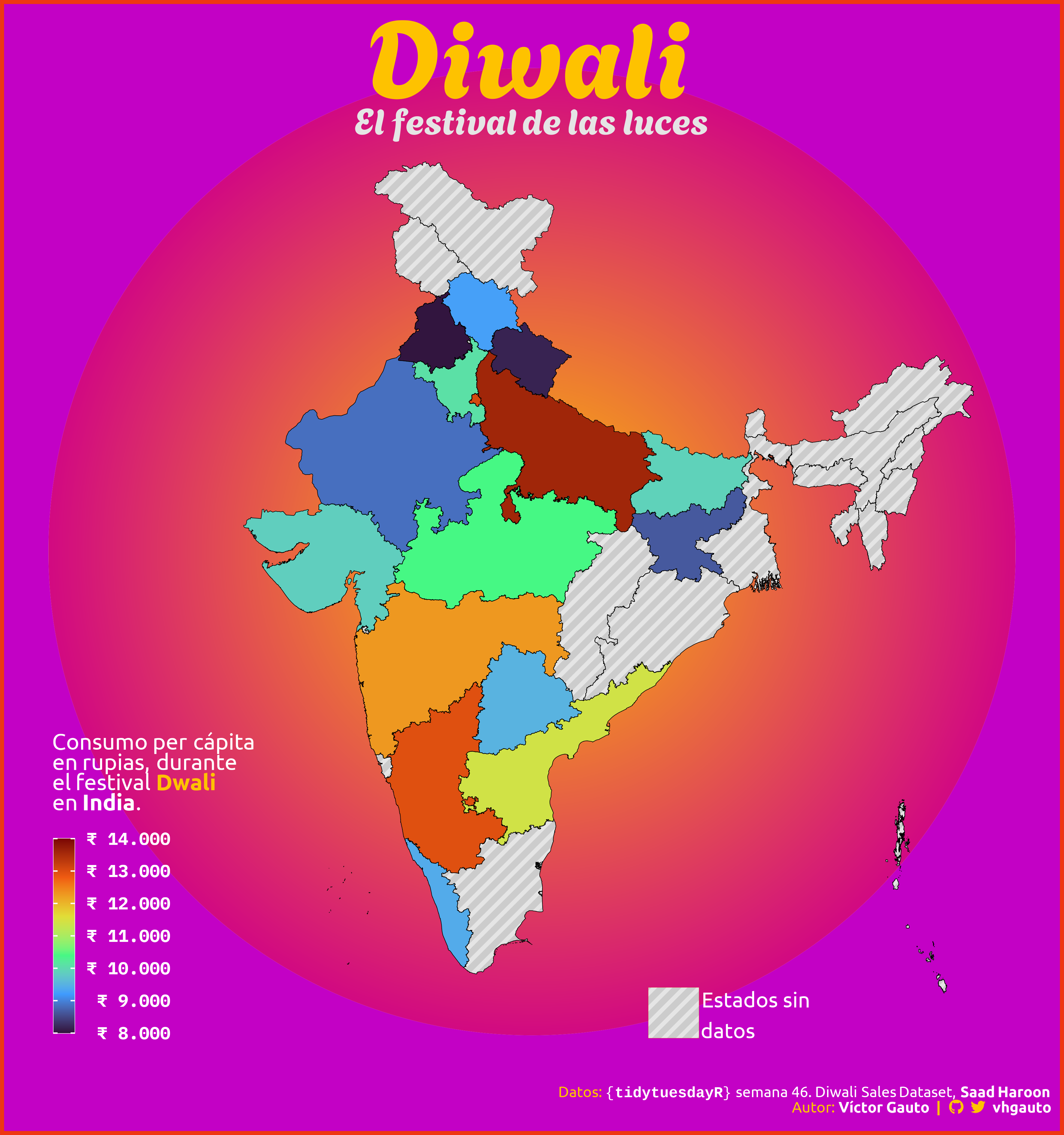
mi_tit <- "Diwali"
mi_tit2 <- "El festival de las luces"
mi_sub <- glue(
"Consumo per cápita",
"en rupias, durante",
"el festival <b style='color:{c1}'>Dwali</b>",
"en **India**.",
.sep = "<br>")
# figura
g <- ggplot() +
# círculo de fondo
geom_sf_pattern(
data = circ,
color = NA, pattern = "gradient",
pattern_orientation = "radial",
pattern_fill = c1, # centro
pattern_fill2 = c5, # exterior
pattern_density = 1) +
# India
geom_sf(data = d_sf, aes(fill = prom), color = NA) +
# estados sin datos
geom_sf_pattern(
data = d_na, pattern = "stripe", show.legend = FALSE, color = NA,
fill = c8, pattern_spacing = 0.01, pattern_density = 0.4,
pattern_fill = c9, pattern_color = NA, pattern_angle = 45) +
# contorno de los estados
geom_sf(data = d_sf, fill = NA, color = "black", linewidth = .2) +
# caja
geom_sf_pattern(
data = caja, pattern = "stripe", show.legend = FALSE, color = c4,
fill = c8, pattern_spacing = 0.01, pattern_density = 0.4,
pattern_fill = c9, pattern_color = NA, pattern_angle = 45,
linewidth = .1) +
annotate(
geom = "text", x = xmax+10000, y = ymin, label = "Estados sinndatos",
hjust = 0, vjust = 0, family = "ubuntu", color = "white", size = 6) +
# título
annotate(
geom = "richtext", x = 3943500, y = 5590000, label = mi_tit, size = 30,
family = "agbalumo", hjust = .5, vjust = 0, color = c1, fill = NA,
label.color = NA) +
annotate(
geom = "richtext", x = 3943500, y = 5670000, label = mi_tit2, size = 10,
family = "agbalumo", hjust = .5, vjust = 1, color = c9, fill = NA,
label.color = NA) +
coord_sf(clip = "off") +
scale_fill_viridis_c(
option = "turbo", na.value = NA, limits = c(8000, 14000),
labels = scales::label_dollar(
big.mark = ".", decimal.mark = ",", prefix = "₹ ", scale = 1)) +
labs(caption = mi_caption, fill = mi_sub) +
guides(
fill = guide_colorbar(
frame.colour = "white", ticks.colour = "white", ticks.linewidth = .5)) +
theme_void() +
theme(
plot.background = element_rect(fill = c6, color = c7, linewidth = 3),
plot.margin = margin(15.7, 0, 5.7, 0),
plot.title = element_text(
family = "playball", size = 55, color = c1, margin = margin(15, 0, 0, 0)),
plot.caption = element_markdown(
family = "ubuntu", color = c1, margin = margin(0, 10, 10, 0), size = 12),
legend.position = c(.05, .05),
legend.justification = c(0, 0),
legend.text = element_text(
hjust = 1, family = "ibm", color = "white", face = "bold", size = 14),
legend.title = element_markdown(
family = "ubuntu", color = "white", size = 18,
margin = margin(0, 0, 10, 0)),
legend.key.height = unit(1.1, "cm"))
# guardo
ggsave(
plot = g,
filename = "2023/semana_46/viz.png",
width = 30,
height = 32,
units = "cm")
# abro
browseURL("2023/semana_46/viz.png")