Ocultar código
library(glue)
library(ggtext)
library(showtext)
library(tidyverse)Cantidad de nutrientes en platos de cinco países.
library(glue)
library(ggtext)
library(showtext)
library(tidyverse)Colores.
c1 <- "#D8DEE9"
c2 <- "#2E3440"
c3 <- "#3B4252"
c4 <- "#434C5E"
c5 <- "white"
c6 <- "#74ACDF"
Fuentes: Ubuntu y JetBrains Mono.
font_add(
  family = "ubuntu",
  regular = "././fuente/Ubuntu-Regular.ttf",
  bold = "././fuente/Ubuntu-Bold.ttf",
  italic = "././fuente/Ubuntu-Italic.ttf"
)

font_add(
  family = "jet",
  regular = "././fuente/JetBrainsMonoNLNerdFontMono-Regular.ttf"
)

showtext_auto()
showtext_opts(dpi = 300)fuente <- glue(
"Datos: <span style='color:{c1};'><span style='font-family:jet;'>",
"{{<b>tidytuesdayR</b>}}</span> semana 37, ",
"<b>{{tastyR}}, allrecipes.com</b></span>"
)
autor <- glue("<span style='color:{c1};'>**Víctor Gauto**</span>")
icon_twitter <- glue("<span style='font-family:jet;'></span>")
icon_instagram <- glue("<span style='font-family:jet;'></span>")
icon_github <- glue("<span style='font-family:jet;'></span>")
icon_mastodon <- glue("<span style='font-family:jet;'>󰫑</span>")
icon_bsky <- glue("<span style='font-family:jet;'></span>")
usuario <- glue("<span style='color:{c1};'>**vhgauto**</span>")
sep <- glue("**|**")
mi_caption <- glue(
"{fuente}<br>{autor} {sep} {icon_github} {icon_twitter} {icon_instagram} ",
"{icon_mastodon} {icon_bsky} {usuario}"
)tuesdata <- tidytuesdayR::tt_load(2025, 37)
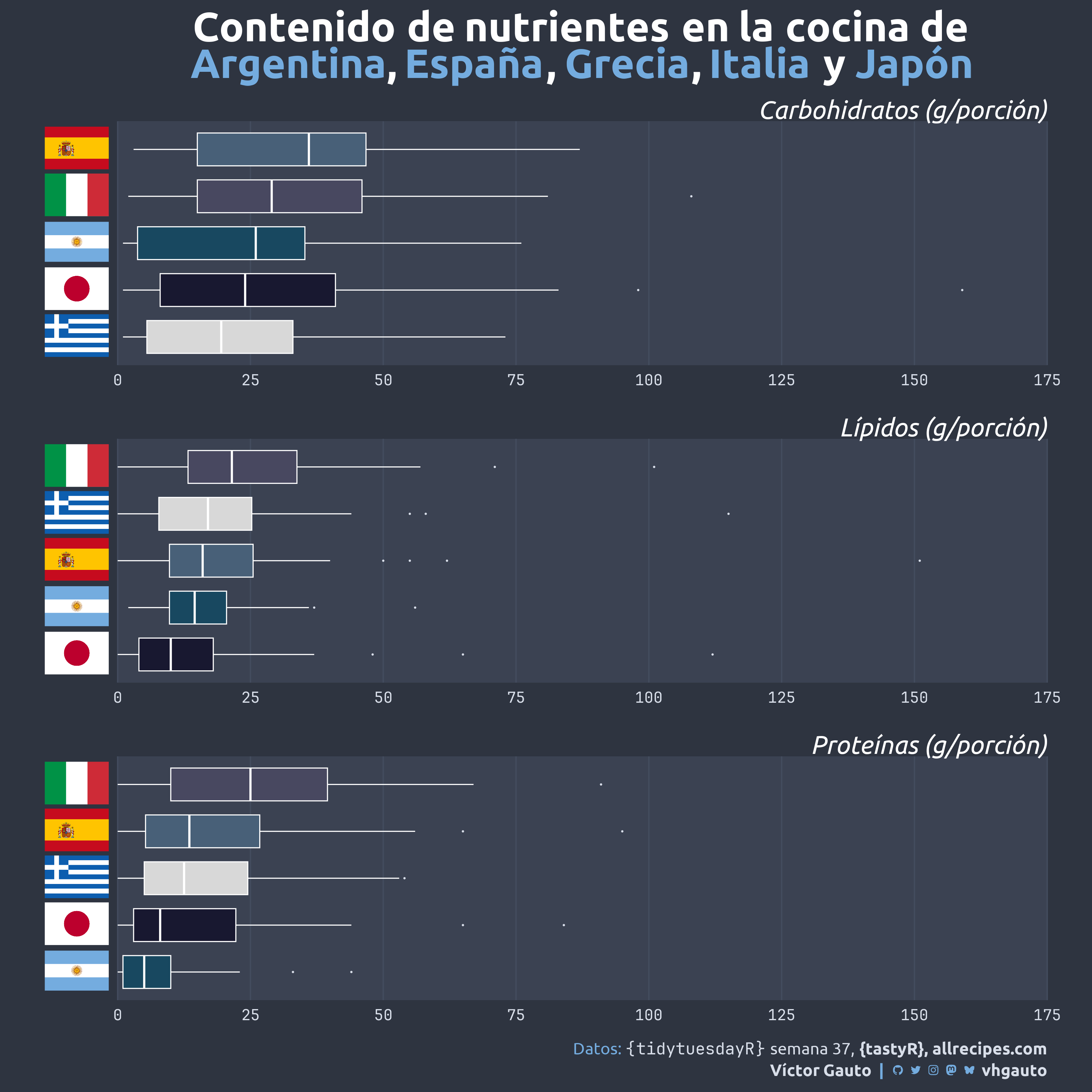
cuisines <- tuesdata$cuisinesMe interesa la distribución de la cantidad de nutrientes (lípidos, carbohidratos y proteínas) en cinco países (Argentina, Grecia, Italia, Japón y España).
Creo etiquetas para nutrientes y países.
nut_tbl <- tibble(
  nut = c("fat", "carbs", "protein"),
  nut_trad = c(
    "Lípidos (g/porción)",
    "Carbohidratos (g/porción)",
    "Proteínas (g/porción)"
  )
)

country_tbl <- tibble(
  country = c("argentinian", "greek", "italian", "japanese", "spanish"),
  pais = c("Argentina", "Grecia", "Italia", "Japón", "España"),
  sym = c("AR", "GR", "IT", "JP", "ES")
)
Filtro por países e incorporo las banderas.
link <- "<img src='https://raw.githubusercontent.com/fonttools/region-flags/refs/heads/gh-pages/png/"

d <- cuisines |>
  mutate(country = tolower(country)) |>
  filter(str_detect(country, "arg|spa|ital|greek|japan")) |>
  select(name, country, calories, fat, carbs, protein, avg_rating) |>
  pivot_longer(
    cols = fat:protein,
    values_to = "valor",
    names_to = "nut"
  ) |>
  drop_na() |>
  full_join(nut_tbl, by = join_by(nut)) |>
  full_join(country_tbl, by = join_by(country)) |>
  mutate(flag = paste0(link, sym, ".png' width=50></img>")) |>
mutate(flag = fct_reorder(flag, valor))Etiquetas de los países y título.
pais_label <- str_flatten_comma(
  paste0("<b style='color:", c6, ";'>", sort(country_tbl$pais), "</b>"),
  last = " y "
)

mi_titulo <- glue(
  "Contenido de nutrientes en la cocina de<br>{pais_label}"
)
Figura.
g <- ggplot(
  d,
  aes(
    x = valor,
    y = tidytext::reorder_within(flag, valor, nut_trad, median),
    fill = pais
  )
) +
  geom_boxplot(
    color = c5,
    width = .7,
    linewidth = .4,
    outlier.color = c1,
    outlier.size = .2
  ) +
  facet_wrap(vars(nut_trad), scales = "free_y", ncol = 1, axes = "all_x") +
  nord::scale_fill_nord(palette = "mountain_forms") +
  tidytext::scale_y_reordered() +
  scale_x_continuous(
    breaks = scales::breaks_width(25),
    limits = c(0, 175),
    expand = c(0, 0)
  ) +
  coord_cartesian(clip = "off", expand = TRUE) +
  labs(x = NULL, y = NULL, title = mi_titulo, caption = mi_caption) +
  ggridges::theme_ridges(font_size = 15, font_family = "ubuntu") +
  theme(
    plot.background = element_rect(fill = c2),
    plot.margin = margin(r = 35, l = 35, b = 10, t = 10),
    plot.title = element_markdown(
      size = 32,
      color = c5,
      hjust = .5,
      margin = margin(b = 10)
    ),
    plot.title.position = "panel",
    plot.caption = element_markdown(
      size = 13,
      color = c6,
      lineheight = 1.3,
      margin = margin(t = 15)
    ),
    panel.background = element_rect(fill = c3),
    panel.spacing.y = unit(22, "pt"),
    panel.grid.major.y = element_blank(),
    panel.grid.major.x = element_line(color = c4),
    legend.position = "none",
    axis.text = element_text(color = c1, family = "jet", size = 12),
    axis.text.y = element_markdown(vjust = .5),
    axis.ticks = element_blank(),
    strip.background = element_blank(),
    strip.text = element_text(
      size = 20,
      hjust = 1,
      face = "italic",
      color = c5
    ),
    strip.clip = "off"
  )
Guardo.
ggsave(
  plot = g,
  filename = "tidytuesday/2025/semana_37.png",
  width = 30,
  height = 30,
  units = "cm"
)