Ocultar código
library(glue)
library(ggtext)
library(showtext)
library(osmdata)
library(sf)
library(patchwork)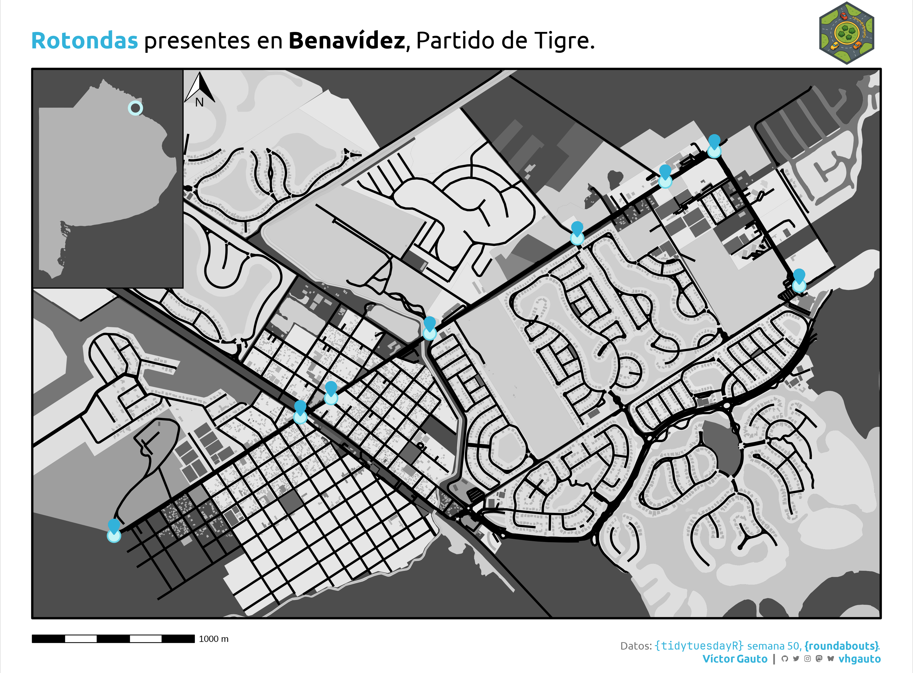
library(tidyverse)Rotondas presentes en Benavidez, Partido de Tigre, Provincia de Buenos Aires.
library(glue)
library(ggtext)
library(showtext)
library(osmdata)
library(sf)
library(patchwork)
library(tidyverse)Colores.
cel <- c("#c3f4f6", "#6ad5e8", "#32b2da")
cc <- rev(grey.colors(14))
Fuentes: Ubuntu y JetBrains Mono.
font_add(
  family = "ubuntu",
  regular = "././fuente/Ubuntu-Regular.ttf",
  bold = "././fuente/Ubuntu-Bold.ttf",
  italic = "././fuente/Ubuntu-Italic.ttf"
)

font_add(
  family = "jet",
  regular = "././fuente/JetBrainsMonoNLNerdFontMono-Regular.ttf"
)

showtext_auto()
showtext_opts(dpi = 300)fuente <- glue(
"Datos: <span style='color:{cel[3]};'><span style='font-family:jet;'>",
"{{<b>tidytuesdayR</b>}}</span> semana 50, ",
"<b>{{roundabouts}}</b>.</span>"
)
autor <- glue("<span style='color:{cel[3]};'>**Víctor Gauto**</span>")
icon_twitter <- glue("<span style='font-family:jet;'></span>")
icon_instagram <- glue("<span style='font-family:jet;'></span>")
icon_github <- glue("<span style='font-family:jet;'></span>")
icon_mastodon <- glue("<span style='font-family:jet;'>󰫑</span>")
icon_bsky <- glue("<span style='font-family:jet;'></span>")
usuario <- glue("<span style='color:{cel[3]};'>**vhgauto**</span>")
sep <- glue("**|**")
mi_caption <- glue(
"{fuente}<br>{autor} {sep} {icon_github} {icon_twitter} {icon_instagram} ",
"{icon_mastodon} {icon_bsky} {usuario}"
)tuesdata <- tidytuesdayR::tt_load(2025, 50)
roundabouts <- tuesdata$roundabouts_cleanMe interesa crear un mapa de Benavidez mostrando las rotondas presentes. Los componentes del mapa provienen de Open Street Map.
Creo funciones para obtener los datos y luego recortar y extraer los vectores.
f_osm <- function(KEY) {
  opq(bbox = st_bbox(v)) |>
    add_osm_feature(key = KEY) |>
    osmdata_sf()
}

f_sf <- function(vector, geometria) {
  vector[[paste0("osm_", geometria)]] |>
    st_geometry() |>
    st_crop(bb)
}
Defino las rotondas de interés y obtengo su extensión.
v <- roundabouts |>
  filter(country == "Argentina" & town_city == "Benavídez") |>
  st_as_sf(coords = c("lat", "long"), crs = "EPSG:4326") |>
  st_geometry()

bb <- st_buffer(v, dist = 500) |>
  st_bbox() |>
  st_as_sfc()
Obtengo los vectores de los componentes de la región de interés.
osm_camino <- f_osm("highway") |>
  f_sf("lines")
osm_agua1 <- f_osm("water") |>
  f_sf("multipolygons")
osm_agua2 <- f_osm("waterway") |>
  f_sf("multilines")
osm_natural1 <- f_osm("natural") |>
  f_sf("multipolygons")
osm_natural2 <- f_osm("natural") |>
  f_sf("polygons")
osm_edificio1 <- f_osm("building") |>
  f_sf("polygons")
osm_edificio2 <- f_osm("building") |>
  f_sf("multipolygons")
osm_suelo1 <- f_osm("landuse") |>
  f_sf("polygons")
osm_suelo2 <- f_osm("landuse") |>
  f_sf("multipolygons")
osm_amenity1 <- f_osm("amenity") |>
  f_sf("multipolygons")
osm_amenity2 <- f_osm("amenity") |>
  f_sf("polygons")
osm_tienda1 <- f_osm("shop") |>
  f_sf("polygons")
osm_ocio1 <- f_osm("leisure") |>
  f_sf("multipolygons")
osm_ocio2 <- f_osm("leisure") |>
f_sf("polygons")Vector y mapa de la Provincia de Buenos Aires.
bsas <- geoAr::get_geo("BUENOS AIRES") |>
  st_geometry() |>
  st_union()

g_bsas <- ggplot() +
  geom_sf(data = bsas, fill = cc[7], color = NA) +
  geom_sf(
    data = st_centroid(bb),
    fill = cc[14],
    size = 4,
    shape = 21,
    color = cel[1],
    stroke = 2
  ) +
  theme_void() +
  theme_sub_plot(
    background = element_rect(fill = cc[14], color = "black", linewidth = 1),
    margin = margin_auto(0)
  )
Logo del paquete {roundabouts} que contiene los datos. Creo un tibble para luego incorporar la figura.
logo_url <- "https://raw.githubusercontent.com/EmilHvitfeldt/roundabouts/refs/heads/main/man/figures/logo.png"
logo_tbl <- tibble(
  image = logo_url,
  x = I(.96),
  y = I(1.065)
)
Utilizo el símbolo
pin_url <- "https://api.iconify.design/fa6-solid/location-pin.svg?color=%2332b2da"
pin_txt <- paste(readLines(pin_url), collapse = "\n")
pin_tbl <- as_tibble(st_coordinates(v))
Título y mapa principal.
mi_titulo <- glue(
  "<b style='color:{cel[3]}'>Rotondas</b> presentes en **Benavídez**,
  Partido de Tigre."
)

g <- ggplot() +
  geom_sf(data = bb, fill = cc[14], color = NA, linewidth = 1) +
  geom_sf(data = osm_suelo1, fill = cc[1], color = NA) +
  geom_sf(data = osm_suelo2, fill = cc[2], color = NA) +
  geom_sf(data = osm_natural1, fill = cc[3], color = NA) +
  geom_sf(data = osm_natural2, fill = cc[4], color = NA) +
  geom_sf(data = osm_agua1, fill = cc[5], color = NA) +
  geom_sf(data = osm_agua2, fill = cc[6], color = cc[6]) +
  geom_sf(data = osm_edificio1, fill = cc[7], color = NA) +
  geom_sf(data = osm_edificio2, fill = cc[8], color = NA) +
  geom_sf(data = osm_amenity1, fill = cc[9], color = NA) +
  geom_sf(data = osm_amenity2, fill = cc[10], color = NA) +
  geom_sf(data = osm_camino, color = "black", linewidth = 1) +
  geom_sf(data = osm_tienda1, fill = cc[11], color = NA) +
  geom_sf(data = osm_ocio1, fill = cc[12], color = NA) +
  geom_sf(data = osm_ocio2, fill = cc[13], color = NA) +
  geom_sf(
    data = v,
    fill = cel[1],
    color = cel[2],
    shape = 21,
    size = 5,
    stroke = 1
  ) +
  ggsvg::geom_point_svg(
    data = pin_tbl,
    aes(X, Y + .0005),
    svg = pin_txt,
    size = 4
  ) +
  ggimage::geom_image(data = logo_tbl, aes(x, y, image = image), size = .1) +
  geom_sf(data = bb, fill = NA, color = "black", linewidth = 1) +
  ggspatial::annotation_scale(
    location = "bl",
    pad_x = unit(0., "cm"),
    pad_y = unit(-.8, "cm"),
    text_col = "black"
  ) +
  ggspatial::annotation_north_arrow(
    location = "tl",
    pad_x = unit(5, "cm"),
    pad_y = unit(.1, "cm"),
    height = unit(1.1, "cm"),
    width = unit(1, "cm"),
  ) +
  coord_sf(expand = FALSE, clip = "off") +
  labs(title = mi_titulo, caption = mi_caption) +
  theme_void(base_family = "ubuntu") +
  theme_sub_plot(
    title = element_markdown(hjust = 0, size = 22, margin = margin(b = 15)),
    caption = element_markdown(
      color = cc[12],
      size = 10,
      lineheight = 1.2,
      margin = margin(b = -22, t = 22)
    )
  )
Composición del mapa principal con el mapa de Buenos Aires.
g_mapa <- g +
  inset_element(g_bsas, -0.022, 0.6, .2, 1) +
  plot_annotation(theme = theme_sub_plot(margin = margin_auto(30)))
Guardo.
ggsave(
  plot = ,
  filename = "tidytuesday/2025/semana_50.png",
  width = 30,
  height = 22.14,
  units = "cm"
)