Ocultar código
library(glue)
library(ggtext)
library(showtext)
library(tidyverse)Nombres más populares de gatos y perros.
library(glue)
library(ggtext)
library(showtext)
library(tidyverse)Colores.
c1 <- "#6497B1"
c2 <- "#FFF2F5"
c3 <- "#6A359C"
c4 <- "#679C35"
Fuentes: Ubuntu y JetBrains Mono.
font_add(
  family = "ubuntu",
  regular = "././fuente/Ubuntu-Regular.ttf",
  bold = "././fuente/Ubuntu-Bold.ttf",
  italic = "././fuente/Ubuntu-Italic.ttf"
)

font_add(
  family = "jet",
  regular = "././fuente/JetBrainsMonoNLNerdFontMono-Regular.ttf"
)

font_add(
  family = "bebas",
  regular = "././fuente/BebasNeue-Regular.ttf"
)

showtext_auto()
showtext_opts(dpi = 300)fuente <- glue(
"Datos: <span style='color:{c1};'><span style='font-family:jet;'>",
"{{<b>tidytuesdayR</b>}}</span> semana 09, ",
"<b>{{animalshelter}}</b>.</span>"
)
autor <- glue("<span style='color:{c1};'>**Víctor Gauto**</span>")
icon_twitter <- glue("<span style='font-family:jet;'></span>")
icon_instagram <- glue("<span style='font-family:jet;'></span>")
icon_github <- glue("<span style='font-family:jet;'></span>")
icon_mastodon <- glue("<span style='font-family:jet;'>󰫑</span>")
icon_bsky <- glue("<span style='font-family:jet;'></span>")
usuario <- glue("<span style='color:{c1};'>**vhgauto**</span>")
sep <- glue("**|**")
mi_caption <- glue(
"{fuente}<br>{autor} {sep} {icon_github} {icon_twitter} {icon_instagram} ",
"{icon_mastodon} {icon_bsky} {usuario}"
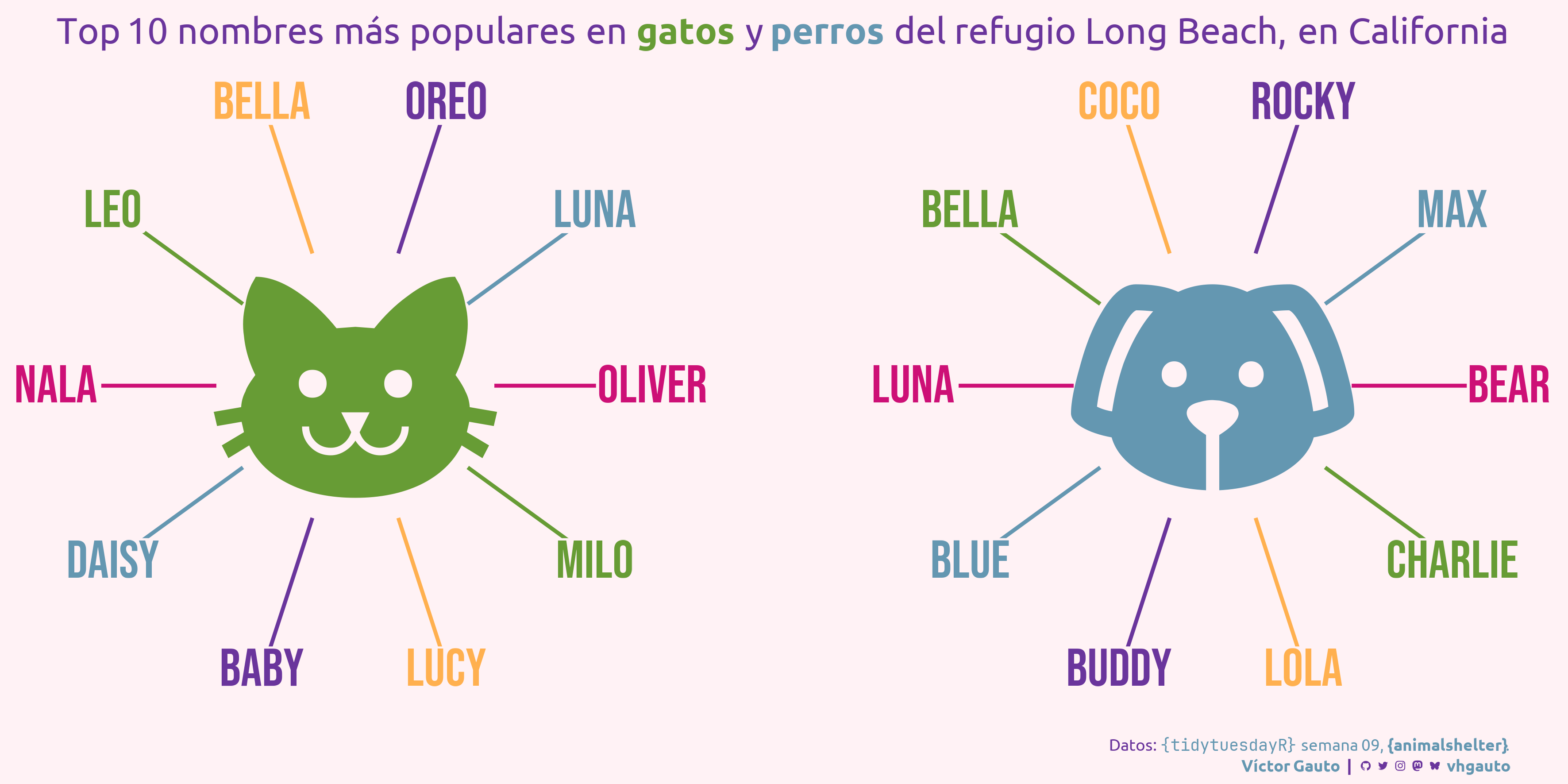
)tuesdata <- tidytuesdayR::tt_load(2025, 09)
longbeach <- tuesdata$longbeachMe interesan los nombres más populares en perros y gatos.
nombres <- longbeach |>
  select(animal_name, animal_type) |>
  filter(!str_detect(animal_name, fixed("*"))) |>
  filter(animal_name != "unknown") |>
  filter(!str_detect(animal_name, "kitten")) |>
  count(animal_name, animal_type) |>
  slice_max(order_by = n, n = 10, by = animal_type, with_ties = FALSE) |>
  filter(animal_type %in% c("dog", "cat")) |>
  select(-n, "nombre" = animal_name, "tipo" = animal_type)
Dispongo los nombres de manera radial.
radio <- 1

d <- nombres |>
  mutate(
    id = row_number(), .by = tipo
  ) |>
  mutate(
    alfa = id/max(id)*2*pi
  ) |>
  mutate(
    x = radio*cos(alfa),
    y = radio*sin(alfa)
  ) |>
  mutate(
    color = rep(PrettyCols::prettycols(palette = "Bold"), 4)
  )
Íconos de perro y gato para ubicar en el centro de cada panel.
icono <- tibble(
x = 0,
y = -.14,
label = c("󰩃", "󰄛"),
tipo = c("dog", "cat"),
color = c(c1, c4)
)Íconos coloreados de perro y gato para usar en el subtítulo.
perros <- glue("<b style='color: {c1}'>perros</b>")
gatos <- glue("<b style='color: {c4}'>gatos</b>")

mi_subtitulo <- glue(
  "Top 10 nombres más populares en {gatos} y {perros} del refugio Long
  Beach, en California"
)
Figura.
g <- ggplot(d, aes(x, y, label = nombre, color = color)) +
  geom_segment(
    aes(x = 0, y = 0, xend = x, yend = y, color = color), linewidth = 1
  ) +
  annotate(
    geom = "point", x = 0, y = 0, size = 70, color = c2
  ) +
  geom_richtext(
    family = "bebas", size = 10, label.color = NA, fill = c2,
    label.padding = unit(.1, "lines")
  ) +
  geom_richtext(
    data = icono, aes(x, y, label = label, color = color), family = "jet",
    fill = NA, label.color = NA, size = 90, inherit.aes = FALSE
  ) +
  facet_wrap(vars(tipo), nrow = 1) +
  scale_color_identity() +
  coord_cartesian(
    clip = "off", expand = FALSE, xlim = c(-1, 1), ylim = c(-1, 1)
  ) +
  labs(subtitle = mi_subtitulo, caption = mi_caption) +
  theme_void() +
  theme(
    aspect.ratio = 1,
    text = element_text(family = "ubuntu", color = c3),
    plot.margin = margin(l = 30, r = 30),
    plot.background = element_rect(fill = c2, color = NA),
    plot.subtitle = element_markdown(
      size = 20, hjust = .5, margin = margin(b = 20, t = 10)
    ),
    plot.caption = element_markdown(
      margin = margin(b = 5, t = 30), lineheight = 1.3
    ),
    panel.spacing.x = unit(5, "cm"),
    panel.background = element_blank(),
    strip.text = element_blank()
  )
Guardo.
ggsave(
  plot = g,
  filename = "tidytuesday/2025/semana_09.png",
  width = 30,
  height = 15,
  units = "cm"
)