# paquetes ----------------------------------------------------------------
library(tidyverse)
library(ggtext)
library(glue)
library(showtext)
library(ggridges)
# fuente ------------------------------------------------------------------
# colores
# paleta 'Homer1' de MetBrewer
c1 <- "#c3f4f6"
c2 <- "#6ad5e8"
c3 <- "#df9ed4"
c4 <- "#16317d"
c5 <- "#a62f00"
# eje vertical, años
font_add_google(name = "Bebas Neue", family = "bebas")
# texto gral
font_add_google(name = "Carlito", family = "carlito", db_cache = FALSE)
# eje horizontal
font_add_google(name = "Inconsolata", family = "inconsolata")
# título
font_add_google(name = "Noto Serif", family = "noto")
showtext_auto()
showtext_opts(dpi = 300)
# íconos
font_add("fa-brands", "icon/Font Awesome 6 Brands-Regular-400.otf")
showtext_auto()
showtext_opts(dpi = 300)
# caption
fuente <- glue("Datos: <span style='color:{c3};'><span style='font-family:mono;'>{{<b>tidytuesdayR</b>}}</span> semana 19</span>")
autor <- glue("Autor: <span style='color:{c3};'>**Víctor Gauto**</span>")
icon_twitter <- glue("<span style='font-family:fa-brands;'></span>")
icon_github <- glue("<span style='font-family:fa-brands;'></span>")
usuario <- glue("<span style='color:{c3};'>**vhgauto**</span>")
sep <- glue("**|**")
mi_caption <- glue("{fuente} {sep} {autor} {sep} {icon_github} {icon_twitter} {usuario}")
# datos -------------------------------------------------------------------
browseURL("https://github.com/rfordatascience/tidytuesday/blob/master/data/2023/2023-05-09/readme.md")
childcare_costs <- readr::read_csv('https://raw.githubusercontent.com/rfordatascience/tidytuesday/master/data/2023/2023-05-09/childcare_costs.csv')
counties <- readr::read_csv('https://raw.githubusercontent.com/rfordatascience/tidytuesday/master/data/2023/2023-05-09/counties.csv')
# acomodo los datos
# selecciono 'infant'
datos <- childcare_costs |>
select(study_year, ends_with("infant"), mhi_2018) |>
pivot_longer(cols = ends_with("infant"),
values_to = "price",
names_to = "group") |>
separate(group, into = c("base", "age"), sep = "_") |>
mutate(study_year = factor(study_year)) |>
select(-age) |>
drop_na(price)
# valores de mediana, por 'base' y 'study_year'
m <- datos |>
group_by(study_year, base) |>
summarise(price = median(price, na.rm = TRUE)) |>
ungroup() |>
mutate(label = format(round(price, 1), nsmall = 1)) |>
mutate(label = str_replace_all(label, "\.", ","))
# figura ------------------------------------------------------------------
g <- ggplot() +
# horizontales en gris
geom_hline(yintercept = factor(2008:2018), color = c2, linewidth = .5) +
# densidad, con fill
geom_density_ridges(
data = datos,
aes(x = price, y = study_year, color = base),
alpha = 0, panel_scaling = FALSE, scale = 1, show.legend = FALSE,
size = 1) +
# punto de mediana
geom_text(
data = m,
aes(x = price, y = study_year, label = "|"),
size = 3, nudge_y = .05, show.legend = FALSE, color = c2) +
# valor de mediana
geom_text(
data = m,
aes(x = price, y = study_year, label = label, color = base),
size = 4, nudge_y = .14, family = "inconsolata", show.legend = FALSE,
fontface = "bold") +
# manual
scale_x_continuous(breaks = seq(0, 500, 100)) +
scale_color_manual(values = c(c3, c4)) +
labs(x = "Costo semanal, de tiempo completo (USD, 2018)", y = NULL,
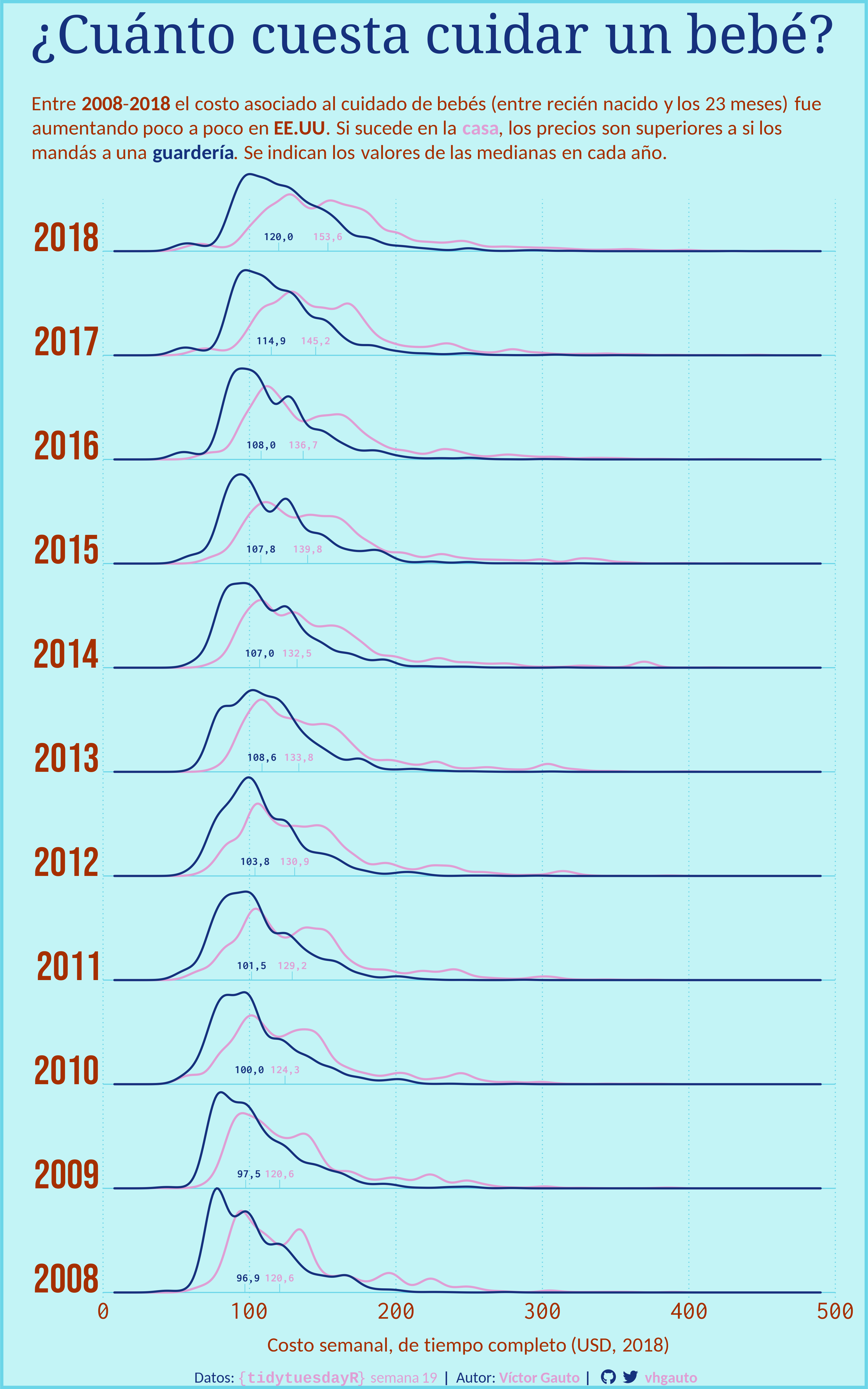
title = "¿Cuánto cuesta cuidar un bebé?",
subtitle = glue(
"Entre **2008**-**2018** el costo asociado al cuidado de bebés (entre recién
nacido y los 23 meses) fue aumentando poco a poco en **EE.UU**. Si sucede
en la <span style='color:{c3};'>**casa**</span>, los precios son superiores a
si los mandás a una <span style='color:{c4};'>**guardería**</span>.
Se indican los valores de las medianas en cada año."),
caption = mi_caption) +
coord_cartesian(expand = FALSE, xlim = c(0, 500), ylim = c(.95, 11.5),
clip = "off") +
theme_minimal() +
theme(
aspect.ratio = 1.5,
plot.background = element_rect(
fill = c1, color = c2, linewidth = 3),
plot.title = element_markdown(
size = 52, family = "noto", color = c4),
plot.title.position = "plot",
plot.subtitle = element_textbox_simple(
size = 20, family = "carlito", color = c5, margin = margin(25, 0, 36, 0)),
plot.caption = element_markdown(
size = 15, color = c4, family = "carlito", hjust = .4,
margin = margin(15, 0, 3, 0)),
plot.margin = margin(15, 32, 0, 32),
panel.background = element_blank(),
panel.grid = element_blank(),
panel.grid.major.x = element_line(color = c2, linewidth = .5, linetype = 3),
axis.text.y = element_text(
size = 40, vjust = 0, family = "bebas", color = c5),
axis.text.x = element_text(
size = 25, family = "inconsolata", color = c5),
axis.title.x = element_markdown(
size = 20, family = "carlito", color = c5, margin = margin(15, 0, 0, 0))
)
# guardo
ggsave(filename = "2023/semana_19/viz.png",
width = 30,
height = 48,
units = "cm",
dpi = 300)
# abro
browseURL("2023/semana_19/viz.png")