Ocultar código
library(glue)
library(ggtext)
library(showtext)
library(tidytext)
library(tidyverse)Palabras más frecuentes en historias de Sherlock Holmes.
library(glue)
library(ggtext)
library(showtext)
library(tidytext)
library(tidyverse)Colores.
c1 <- "#06314E"
c2 <- "#FBE3C2"
c3 <- "#f3ca9f"
c4 <- "#92351d"
c5 <- "#b9563f"
c6 <- "grey20"
c7 <- "grey95"
c8 <- "white"
Fuentes: Ubuntu y JetBrains Mono.
font_add(
  family = "ubuntu",
  regular = "././fuente/Ubuntu-Regular.ttf",
  bold = "././fuente/Ubuntu-Bold.ttf",
  italic = "././fuente/Ubuntu-Italic.ttf"
)

font_add(
  family = "jet",
  regular = "././fuente/JetBrainsMonoNLNerdFontMono-Regular.ttf",
  bold = "././fuente/JetBrainsMonoNLNerdFontMono-Bold.ttf"
)

font_add_google(name = "Tangerine", family = "tangerine")

showtext_auto()
showtext_opts(dpi = 300)fuente <- glue(
"Datos: <span style='color:{c1};'><span style='font-family:jet;'>",
"{{<b>tidytuesdayR</b>}}</span> semana 46, ",
"<b>{{sherlock}}</b>, Emil Hvitfeldt.</span>"
)
autor <- glue("<span style='color:{c1};'>**Víctor Gauto**</span>")
icon_twitter <- glue("<span style='font-family:jet;'></span>")
icon_instagram <- glue("<span style='font-family:jet;'></span>")
icon_github <- glue("<span style='font-family:jet;'></span>")
icon_mastodon <- glue("<span style='font-family:jet;'>󰫑</span>")
icon_bsky <- glue("<span style='font-family:jet;'></span>")
usuario <- glue("<span style='color:{c1};'>**vhgauto**</span>")
sep <- glue("**|**")
mi_caption <- glue(
"{fuente}<br>{autor} {sep} {icon_github} {icon_twitter} {icon_instagram} ",
"{icon_mastodon} {icon_bsky} {usuario}"
)tuesdata <- tidytuesdayR::tt_load(2025, 46)
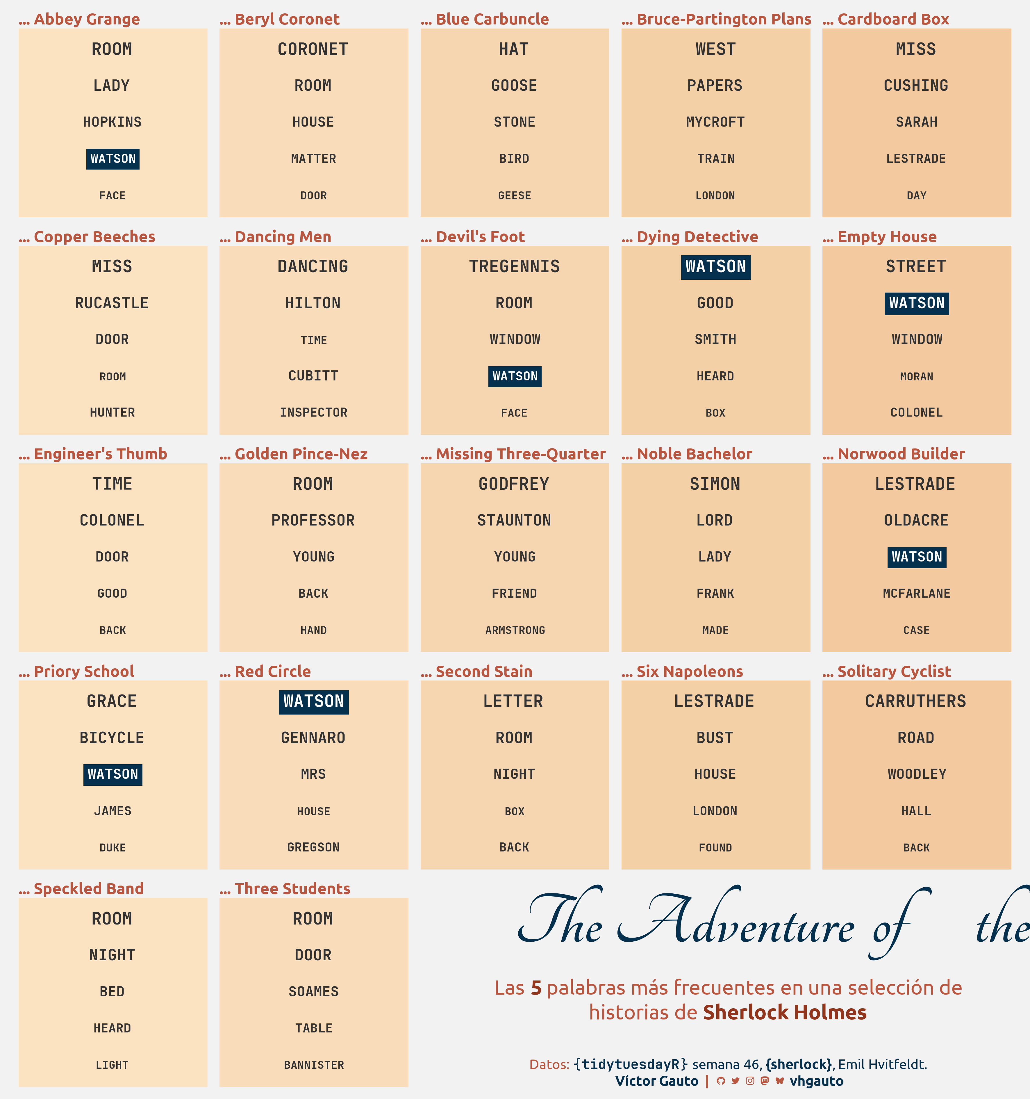
holmes <- tuesdata$holmesMe interesan las cinco palabras más frecuentes en cada libro. En particular, de aquellos libros que comiencen con The Adventure of the…
Creo un tibble con palabras vacías, incluyendo una selección de palabras específicas, como el nombre del protagonista.
sw <- filter(tidytext::stop_words, lexicon == "SMART") |>
  select(-lexicon, palabras = word) |>
  add_row(palabras = c("mr", "st", "dr", "man", "sir", "busts", "holmes"))
Filtro los datos con los libros que me interesan y los renombro. Separo las palabras y obtengo la frecuencia de cada una, por libro, y selecciono las cinco más frecuentes. Agrego formato especial para Watson.
d <- filter(holmes, str_detect(book, "The Adventure of the ")) |>
  mutate(book_label = str_remove(book, "The Adventure of the ")) |>
  mutate(book_label = paste0("... ", book_label)) %>%
  arrange(book) |>
  mutate(book_label = fct_inorder(book_label)) |>
  drop_na(text) |>
  unnest_tokens(output = "palabras", input = "text") |>
  count(palabras, book_label) |>
  drop_na() |>
  anti_join(sw, by = join_by(palabras)) |>
  slice_max(order_by = n, by = book_label, n = 5, with_ties = FALSE) |>
  mutate(palabras = toupper(palabras)) %>%
  mutate(tamaño = rep_len(seq(14, 9, length.out = 5), length.out = nrow(.))) |>
  mutate(
    palabras = glue("<b style='font-size:{tamaño}pt;'>{palabras}</b>")
  ) |>
  mutate(fill = if_else(str_detect(palabras, "WATSON"), c1, NA)) |>
mutate(color = if_else(str_detect(palabras, "WATSON"), c8, c6))Agrego color a cada panel a partir de una rampa de colores.
col <- c(c2, c3)

cuadro <- distinct(d, book_label) |>
  arrange(book_label) %>%
  mutate(fill = rep(colorRampPalette(col)(5), length.out = nrow(.)))
Título y subtítulo.
mi_titulo <- glue("The Adventure of<span style='color:{c7};'>...</span>the...")
mi_subtitulo <- glue(
  "Las <b style='color: {c4}'>5</b> palabras más frecuentes en una ",
  "selección de<br>historias de <b style='color: {c4}'>Sherlock Holmes</b>"
)
Figura.
g <- ggplot(
  d,
  aes(1, reorder_within(palabras, n, book_label), label = palabras)
) +
  geom_rect(
    data = cuadro,
    aes(ymin = -Inf, ymax = Inf, xmin = -Inf, xmax = Inf, fill = fill),
    inherit.aes = FALSE
  ) +
  geom_richtext(
    aes(fill = fill, color = color),
    label.color = NA,
    family = "jet",
    label.r = unit(0, "pt")
  ) +
  annotate(
    geom = "richtext",
    x = I(c(.5, 2.7, 2.7)),
    y = I(c(.85, .45, .07)),
    fill = NA,
    label.color = NA,
    label = c(mi_titulo, mi_subtitulo, mi_caption),
    family = c("tangerine", "ubuntu", "ubuntu"),
    fontface = c("bold", "plain", "plain"),
    size = c(22, 6, 4),
    layout = 22,
    color = c(c1, c5, c5),
    hjust = c(-.3, .5, .5)
  ) +
  facet_wrap(vars(book_label), nrow = 5, scales = "free") +
  scale_y_reordered(labels = 5:1) +
  scale_fill_identity() +
  scale_color_identity() +
  coord_cartesian(clip = "off") +
  theme_void(base_size = 10) +
  theme(aspect.ratio = 1) +
  theme_sub_plot(
    background = element_rect(fill = c7),
    margin = margin_auto(10)
  ) +
  theme_sub_panel(spacing = unit(10, "pt")) +
  theme_sub_strip(
    text = element_text(
      face = "bold",
      family = "ubuntu",
      size = rel(1.3),
      hjust = 0,
      color = c5,
      margin = margin(b = 2)
    ),
    clip = "off"
  )
Guardo.
ggsave(
  plot = g,
  filename = "tidytuesday/2025/semana_46.png",
  width = 30,
  height = 32,
  units = "cm"
)