Semana 28

Figura semana 28

Valores de anomalía de temperatura de la superficie terrestre.

Script

# paquetes ----------------------------------------------------------------

library(tidyverse)
library(glue)
library(ggtext)
library(showtext)

# fuentes -----------------------------------------------------------------

# colores
c1 <- "grey30"
c2 <- "grey70"
c3 <- "white"

# texto gral
font_add_google(name = "Ubuntu", family = "ubuntu")
# anomalías de temperatura
font_add_google(name = "Inconsolata", family = "inconsolata")
# años
font_add_google(name = "Bebas Neue", family = "bebas")
# título
font_add_google(name = "Gloock", family = "gloock", db_cache = FALSE)

# íconos
font_add("fa-brands", "icon/Font Awesome 6 Brands-Regular-400.otf")
font_add("fa-solids", "icon/Font Awesome 6 Free-Solid-900.otf")

showtext_auto()
showtext_opts(dpi = 300)

# caption
fuente <- glue("Datos: <span style='color:{c3};'><span style='font-family:mono;'>{{<b>tidytuesdayR</b>}}</span> semana 28, GISS Surface Temperature Analysis</span>")
autor <- glue("Autor: <span style='color:{c3};'>**Víctor Gauto**</span>")
icon_twitter <- glue("<span style='font-family:fa-brands;'>&#xf099;</span>")
icon_github <- glue("<span style='font-family:fa-brands;'>&#xf09b;</span>")
usuario <- glue("<span style='color:{c3};'>**vhgauto**</span>")
sep <- glue("**|**")

mi_caption <- glue("{fuente} {sep} {autor} {sep} {icon_github} {icon_twitter} {usuario}")

# datos -------------------------------------------------------------------

browseURL("https://github.com/rfordatascience/tidytuesday/blob/master/data/2023/2023-07-11/readme.md")

global_temps <- readr::read_csv('https://raw.githubusercontent.com/rfordatascience/tidytuesday/master/data/2023/2023-07-11/global_temps.csv')

# elijo las anomalía anual (j_d)
d <- global_temps |> 
  janitor::clean_names() |> 
  select(year, j_d) |> 
  drop_na()

# figura ------------------------------------------------------------------

# valores de anomalía de temperatura formateados
anom <- tibble(j_d = seq(-.50, 1.25, .50)) |> 
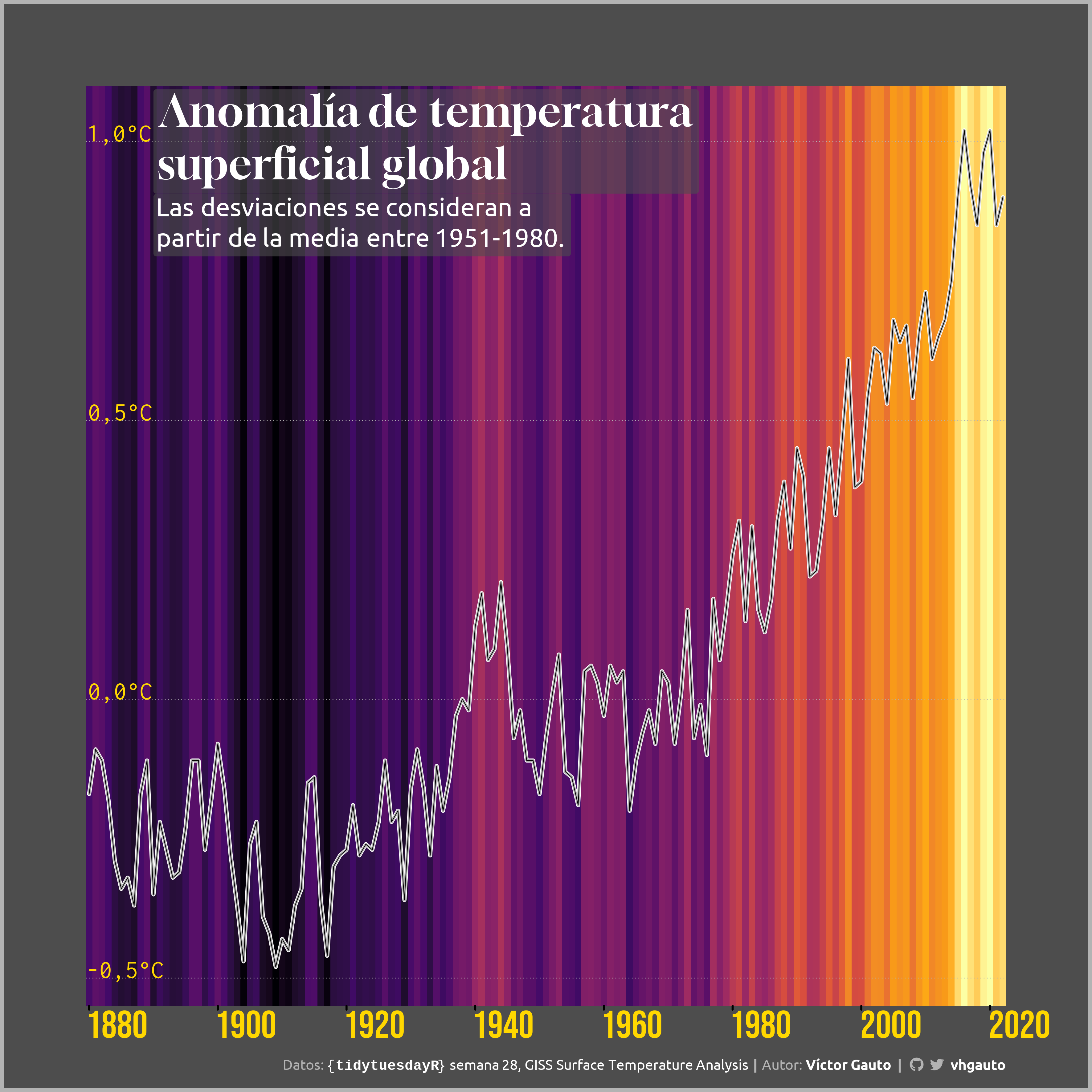
  mutate(label = gt::vec_fmt_number(j_d, decimals = 1, pattern = "{x}°C", sep_mark = ".", dec_mark = ","))

# título de la figura
titulo <- tibble(
  x = 1890,
  y = 1,
  label = "Anomalía de temperatura<br>superficial global"
)

# subtítulo de la figura
subtitulo <- tibble(
  x = 1890,
  y = .85,
  label = "Las desviaciones se consideran a<br>partir de la media entre 1951-1980."
)

# figura
g <- ggplot(data = d, aes(x = year, y = j_d)) +
  # fondo de anomalías
  geom_raster(aes(y = 1, fill = j_d)) +
  geom_raster(aes(y = 0, fill = j_d)) +
  geom_raster(aes(y = -1, fill = j_d)) +
  # horizontales de anomalía de temperatura
  geom_hline(yintercept = anom$j_d, color = c2, linetype = 3, linewidth = .3) +
  # etiquetas de anomalías de temperatura
  geom_text(
    data = anom, aes(x = 1880, y = j_d, label = label), inherit.aes = FALSE,
    angle = 0, hjust = 0, vjust = 0, color = "gold", family = "inconsolata", size = 7) +
  # anomalías de temperatura
  geom_line(linewidth = 1.5, color = "white", lineend = "round") +
  geom_line(linewidth = 1, color = c2, lineend = "round") +
  geom_line(linewidth = .25, color = "black", lineend = "round") +
  # título
  geom_richtext(
    data = titulo, aes(x = x, y = y, label = label), 
    family = "gloock", size = 12, hjust = 0, vjust = .5, fill = alpha(c1, .6),
    label.color = NA, color = c3) +
  # subtítulo
  geom_richtext(
    data = subtitulo, aes(x = x, y = y, label = label), 
    family = "ubuntu", size = 7, hjust = 0, vjust = .5, fill = alpha(c1, .6),
    label.color = NA, color = c3) +
  # maual
  scale_fill_viridis_c(option = "inferno") +
  # ejes
  scale_x_continuous(breaks = seq(1800, 2020, 20)) +
  labs(x = NULL, y = NULL, caption = mi_caption) +
  coord_cartesian(expand = FALSE, ylim = c(-.55, 1.1), clip = "on") +
  theme_void() +
  theme(
    aspect.ratio = 1,
    plot.margin = margin(67, 67, 15, 67),
    plot.background = element_rect(fill = c1, color = c2, linewidth = 3),
    plot.caption.position = "plot",
    plot.caption = element_markdown(
      family = "ubuntu", color = c2, size = 11, margin = margin(15, 0, 0, 0)),
    axis.text.x = element_text(
      color = "gold", family = "bebas", hjust = 0, size = 30),
    axis.ticks.x = element_line(color = "black", linewidth = .75),
    axis.ticks.length.x = unit(.2, "line"),
    legend.position = "none",
    panel.grid = element_blank()
  )

# guardo
ggsave(
    plot = g,
    filename = "2023/semana_28/viz.png",
    width = 30,
    height = 30,
    units = "cm",
    dpi = 300
  )

# abro
browseURL("2023/semana_28/viz.png")

Figura