Ocultar código
library(glue)
library(ggtext)
library(showtext)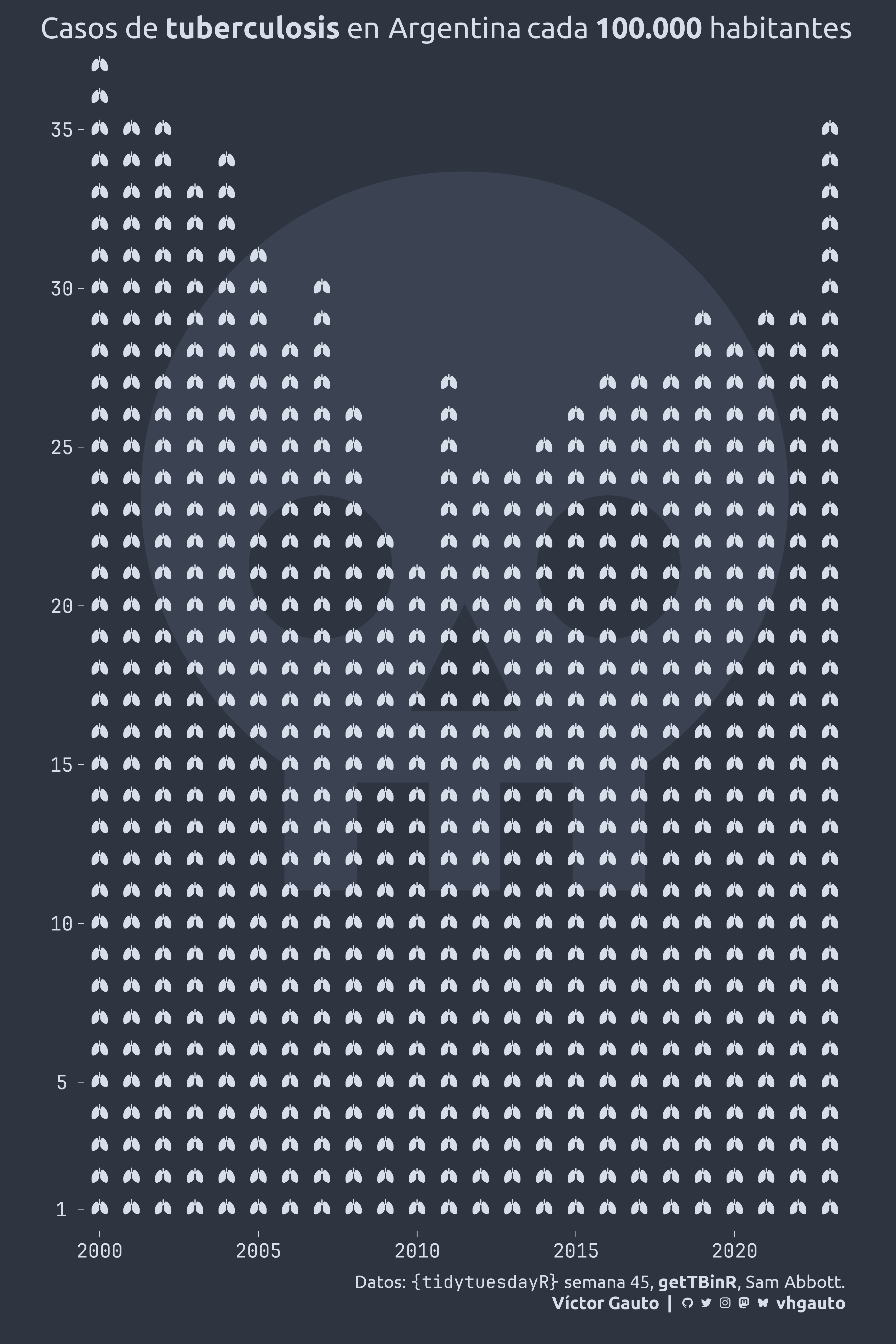
library(tidyverse)Cantidad de casos de tuberculosis cada 100000 habitantes en Argentina.
library(glue)
library(ggtext)
library(showtext)
library(tidyverse)Colores.
col <- nord::nord(palette = "polarnight", n = 4)
c1 <- "#D8DEE9"
c2 <- "#D8DEE9"
Fuentes: Ubuntu y JetBrains Mono.
font_add(
  family = "ubuntu",
  regular = "././fuente/Ubuntu-Regular.ttf",
  bold = "././fuente/Ubuntu-Bold.ttf",
  italic = "././fuente/Ubuntu-Italic.ttf"
)

font_add(
  family = "jet",
  regular = "././fuente/JetBrainsMonoNLNerdFontMono-Regular.ttf"
)

showtext_auto()
showtext_opts(dpi = 300)fuente <- glue(
"Datos: <span style='color:{c1};'><span style='font-family:jet;'>",
"{{<b>tidytuesdayR</b>}}</span> semana 45, ",
"<b>getTBinR</b>, Sam Abbott.</span>"
)
autor <- glue("<span style='color:{c1};'>**Víctor Gauto**</span>")
icon_twitter <- glue("<span style='font-family:jet;'></span>")
icon_instagram <- glue("<span style='font-family:jet;'></span>")
icon_github <- glue("<span style='font-family:jet;'></span>")
icon_mastodon <- glue("<span style='font-family:jet;'>󰫑</span>")
icon_bsky <- glue("<span style='font-family:jet;'></span>")
usuario <- glue("<span style='color:{c1};'>**vhgauto**</span>")
sep <- glue("**|**")
mi_caption <- glue(
"{fuente}<br>{autor} {sep} {icon_github} {icon_twitter} {icon_instagram} ",
"{icon_mastodon} {icon_bsky} {usuario}"
)tuesdata <- tidytuesdayR::tt_load(2025, 45)
who_tb_data <- tuesdata$who_tb_dataMe interesan los casos cada 100000 habitantes en Argentina.
Filtro los datos para Argentina y agrego la columna y con las unidades de cantidad de casos.
d <- filter(who_tb_data, country == "Argentina") |>
  select(year, e_inc_100k) |>
  mutate(l = as.list(e_inc_100k)) |>
  mutate(y = map(l, ~ 1:.x)) |>
  unnest(y)
Defino símbolos para la calavera () y los pulmones ().
calavera <- glue("<span style='font-family:jet;'>󰚌</span>")
pulmón <- glue("<span style='font-family:jet;'></span>")Título y figura.
mi_titulo <- glue(
  "Casos de <b style='color: {c1};'>tuberculosis</b> en Argentina ",
  "cada **100.000** habitantes"
)

g <- ggplot(d, aes(year, y)) +
  annotate(
    geom = "richtext",
    x = I(.5),
    y = I(.5),
    fill = NA,
    label.color = NA,
    label = calavera,
    size = 360,
    color = col[2]
  ) +
  geom_richtext(
    label = pulmón,
    color = c2,
    family = "jet",
    fill = NA,
    label.color = NA,
    size = 9
  ) +
  scale_x_continuous(expand = expansion(mult = 0, add = .5)) +
  scale_y_continuous(
    breaks = c(1, seq(5, 35, 5)),
    expand = expansion(mult = 0, add = .7)
  ) +
  labs(title = mi_titulo, caption = mi_caption) +
  coord_equal() +
  theme_void(base_size = 14, base_family = "ubuntu") +
  theme_sub_legend(position = "none") +
  theme_sub_plot(
    background = element_rect(fill = col[1]),
    title = element_markdown(hjust = .5, size = rel(2), color = c2),
    title.position = "plot",
    margin = margin(b = 15, t = 10),
    caption = element_markdown(
      size = rel(1.2),
      color = c2,
      lineheight = 1.2,
      margin = margin(t = 15, b = 15)
    )
  ) +
  theme_sub_axis(
    text = element_text(color = c1, family = "jet", size = rel(1.3)),
    ticks = element_line(color = c1),
    ticks.length = unit(5, "pt")
  ) +
  theme_sub_axis_y(text = element_text(margin = margin(r = 5))) +
  theme_sub_axis_x(text = element_text(margin = margin(t = 5)))
Guardo.
ggsave(
  plot = g,
  filename = "tidytuesday/2025/semana_45.png",
  width = 30,
  height = 45,
  units = "cm"
)