Ocultar código
library(glue)
library(ggtext)
library(marquee)
library(showtext)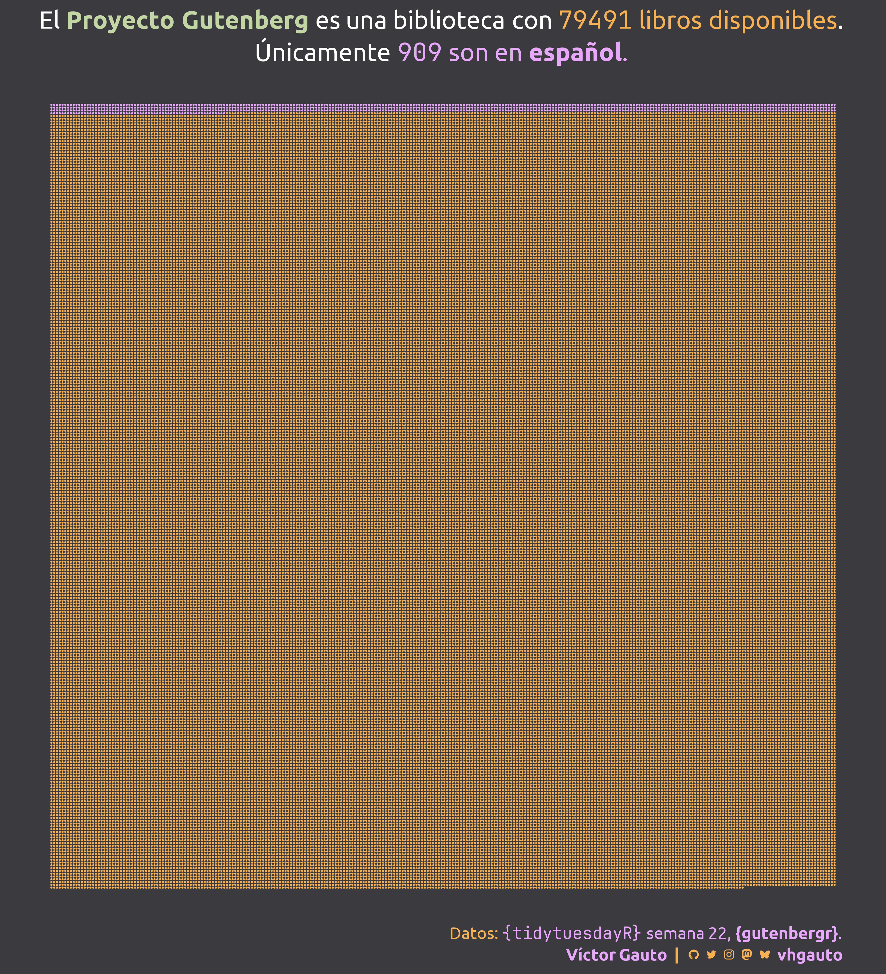
library(tidyverse)Cantidad de libros en español en el Proyecto Gutenberg.
library(glue)
library(ggtext)
library(marquee)
library(showtext)
library(tidyverse)Colores. Remplazo el color rojo con el del logo de Gutenberg.
c1 <- "#E7A8FB"
c2 <- "#F8B150"
c3 <- "#3B3A3E"
c4 <- "#C2D6A4"
Fuentes: Ubuntu y JetBrains Mono.
font_add(
  family = "ubuntu",
  regular = "././fuente/Ubuntu-Regular.ttf",
  bold = "././fuente/Ubuntu-Bold.ttf",
  italic = "././fuente/Ubuntu-Italic.ttf"
)

font_add(
  family = "jet",
  regular = "././fuente/JetBrainsMonoNLNerdFontMono-Regular.ttf"
)

showtext_auto()
showtext_opts(dpi = 300)fuente <- glue(
"Datos: <span style='color:{c1};'><span style='font-family:jet;'>",
"{{<b>tidytuesdayR</b>}}</span> semana 22, ",
"<b>{{gutenbergr}}</b>.</span>"
)
autor <- glue("<span style='color:{c1};'>**Víctor Gauto**</span>")
icon_twitter <- glue("<span style='font-family:jet;'></span>")
icon_instagram <- glue("<span style='font-family:jet;'></span>")
icon_github <- glue("<span style='font-family:jet;'></span>")
icon_mastodon <- glue("<span style='font-family:jet;'>󰫑</span>")
icon_bsky <- glue("<span style='font-family:jet;'></span>")
usuario <- glue("<span style='color:{c1};'>**vhgauto**</span>")
sep <- glue("**|**")
mi_caption <- glue(
"{fuente}<br>{autor} {sep} {icon_github} {icon_twitter} {icon_instagram} ",
"{icon_mastodon} {icon_bsky} {usuario}"
)tuesdata <- tidytuesdayR::tt_load(2025, 22)
gutenberg_metadata <- tuesdata$gutenberg_metadataMe interesa la cantidad de libros en español respecto del total.
n_libros <- nrow(gutenberg_metadata)

n_es <- gutenberg_metadata |>
  filter(language == "es") |>
  nrow()
Defino la cantidad de elementos de cada lado y filtro de acuerdo al idioma.
lado <- round(sqrt(n_libros))

d <- expand_grid(
  y = rev(1:lado),
  x = 1:lado
) |>
  mutate(nro = row_number()) |>
  mutate(español = nro > n_es) |>
filter(nro <= n_libros)Agrego el estilo de los números totales de libros y los que son en español, y defino el título.
n_libros_label <- glue("<span style='font-family: jet'>{n_libros}</span>")
n_es_label <- glue("<span style='font-family: jet'>{n_es}</span>")

mi_titulo <- glue(
  "El <b style='color: {c4}'>Proyecto Gutenberg</b> es una biblioteca con
  <span style='color: {c2}'>**{n_libros_label}** libros disponibles</span>.<br>
  Únicamente <span style='color: {c1}'>{n_es_label} son en **español**.</span>"
)
Figura.
g <- d |>
  ggplot(aes(x, y)) +
  geom_point(aes(color = español), size = .3, show.legend = FALSE) +
  scale_color_manual(
    breaks = c(FALSE, TRUE),
    values = c(c1, c2)
  ) +
  coord_equal() +
  labs(title = mi_titulo, caption = mi_caption) +
  theme_void(base_family = "ubuntu", base_size = 20) +
  theme(
    plot.background = element_rect(fill = c3, color = NA),
    plot.title = element_markdown(
      color = "white",
      lineheight = 1.3,
      hjust = .5
    ),
    plot.caption = element_markdown(
      color = c2,
      margin = margin(b = 10, r = 30),
      lineheight = 1.3
    )
  )
Guardo
ggsave(
  plot = g,
  filename = "tidytuesday/2025/semana_22.png",
  width = 30,
  height = 33,
  units = "cm"
)