Ocultar código
library(glue)
library(ggtext)
library(showtext)
library(tidyterra)
library(terra)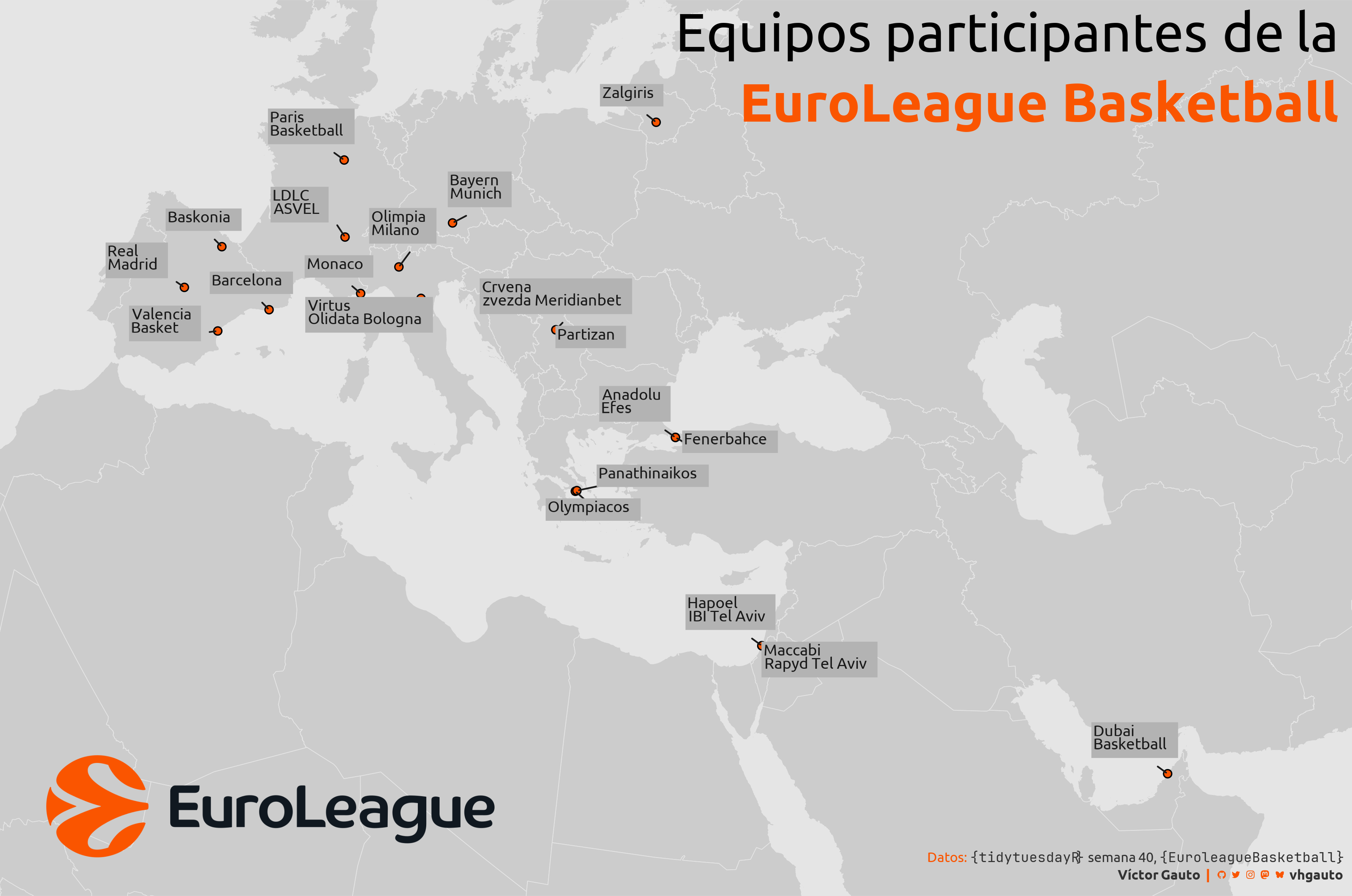
library(tidyverse)Mapa de las ciudades de los equipos de la EuroLeague Basketball.
library(glue)
library(ggtext)
library(showtext)
library(tidyterra)
library(terra)
library(tidyverse)Colores.
c1 <- "#FA5500"
c2 <- "grey90"
c3 <- "grey80"
c4 <- "grey70"
c5 <- "grey50"
c6 <- "grey40"
c7 <- "grey20"
c8 <- "grey10"
c9 <- "black"
Fuentes: Ubuntu y JetBrains Mono.
font_add(
  family = "ubuntu",
  regular = "././fuente/Ubuntu-Regular.ttf",
  bold = "././fuente/Ubuntu-Bold.ttf",
  italic = "././fuente/Ubuntu-Italic.ttf"
)

font_add(
  family = "jet",
  regular = "././fuente/JetBrainsMonoNLNerdFontMono-Regular.ttf"
)

showtext_auto()
showtext_opts(dpi = 300)fuente <- glue(
"Datos: <span style='color:{c7};'><span style='font-family:jet;'>",
"{{<b>tidytuesdayR</b>}}</span> semana 40, ",
"<b style='font-family:jet;'>{{EuroleagueBasketball}}</b>.</span>"
)
autor <- glue("<span style='color:{c7};'>**Víctor Gauto**</span>")
icon_twitter <- glue("<span style='font-family:jet;'></span>")
icon_instagram <- glue("<span style='font-family:jet;'></span>")
icon_github <- glue("<span style='font-family:jet;'></span>")
icon_mastodon <- glue("<span style='font-family:jet;'>󰫑</span>")
icon_bsky <- glue("<span style='font-family:jet;'></span>")
usuario <- glue("<span style='color:{c7};'>**vhgauto**</span>")
sep <- glue("**|**")
mi_caption <- glue(
"{fuente}<br>{autor} {sep} {icon_github} {icon_twitter} {icon_instagram} ",
"{icon_mastodon} {icon_bsky} {usuario}"
)tuesdata <- tidytuesdayR::tt_load(2025, 40)
basketball <- tuesdata$euroleague_basketballMe interesa crear un mapa con las ciudades de los equipos participantes.
Utilizo el paquete ggmap para obtener las coordenadas de los sitios a partir del nombre de la ciudad. Esto requiere contar con el token correspondiente.
ggmap::register_google(key = "XXXXXXXXXX")

d <- basketball |>
  janitor::clean_names() |>
  select(team, home_city) |>
  mutate(coord = ggmap::geocode(home_city)) |>
  unnest(coord)
Convierto los datos a un vector, obtengo el centroide para ubicar el mapa y genero el sistema de referencias ortográfica.
p <- terra::vect(d, geom = c("lon", "lat"), crs = "EPSG:4326")

o <- ext(p) |>
  vect(crs = "EPSG:4326") |>
  centroids()

ox <- terra::geom(o)[1, "x"]
oy <- terra::geom(o)[1, "y"]

ortho_crs <- glue(
  "+proj=ortho +lat_0={oy} +lon_0={oy} +x_0=0 +y_0=0 +R=6371000 +units=m +no_defs +type=crs"
)
Agrego saltos de línea y reproyecto el vector de ciudades.
p$team <- str_replace(p$team, " ", "\n")
p_ortho <- project(p, ortho_crs)
Vector de polígonos de países del mundo, con proyección ortográfica. Identifico los países de las ciudades de los equipos.
w <- rgeoboundaries::geoboundaries() |>
  terra::vect()

w_ortho <- project(w, ortho_crs)

equipo_pais <- intersect(w_ortho, p_ortho)$shapeName

w_ortho$equipo <- w_ortho$shapeName %in% equipo_pais
Extensión para hacer zoom en el mapa, a partir del vector de ciudades de los equipos.
p_ext <- vect(ext(p_ortho) * 1.25, crs = "EPSG:4326") |>
ext()Link y tibble para incorporar el logo.
logo <- "https://upload.wikimedia.org/wikipedia/en/thumb/5/58/EuroLeague.svg/1280px-EuroLeague.svg.png"

logo_tbl <- tibble(
  x = I(.2),
  y = I(.1),
  image = logo
)
Título y figura.
mi_titulo <- glue(
  "Equipos participantes de la<br>",
  "<b style='color: {c1};'>EuroLeague Basketball</b>"
)

g <- ggplot() +
  geom_spatvector(
    data = w_ortho,
    aes(fill = equipo),
    color = c2,
    linetype = 1,
    linewidth = .2,
    show.legend = FALSE
  ) +
  geom_spatvector(
    data = p_ortho,
    shape = 21,
    color = c9,
    fill = c1,
    stroke = .6,
    size = 2
  ) +
  ggrepel::geom_label_repel(
    data = sf::st_as_sf(p_ortho),
    aes(geometry = geometry, label = team),
    stat = "sf_coordinates",
    lineheight = .7,
    label.size = 0,
    label.r = 0,
    size = 3.5,
    min.segment.length = 0,
    color = c8,
    fill = c4,
    family = "ubuntu",
    hjust = 0,
    vjust = 1,
    seed = 2024,
    show.legend = FALSE
  ) +
  ggimage::geom_image(
    data = logo_tbl,
    aes(x, y, image = image),
    size = .5
  ) +
  annotate(
    geom = "richtext",
    label = c(mi_titulo, mi_caption),
    x = I(c(1, 1)),
    y = I(c(1, 0)),
    hjust = 1,
    vjust = c(1, 0),
    family = "ubuntu",
    label.padding = unit(c(.6, .4), "lines"),
    size = c(12, 3),
    fill = NA,
    lineheight = 1.3,
    label.color = NA,
    color = c(c9, c1)
  ) +
  coord_sf(xlim = c(p_ext$xmin, p_ext$xmax), ylim = c(p_ext$ymin, p_ext$ymax)) +
  scale_fill_manual(
    breaks = c(TRUE, FALSE),
    values = c(c6, c3)
  ) +
  theme_void() +
  theme(
    plot.background = element_rect(fill = c2)
  )
Guardo.
ggsave(
  plot = g,
  filename = "tidytuesday/2025/semana_40.png",
  width = 30,
  height = 19.9,
  units = "cm"
)