Ocultar código
library(glue)
library(ggtext)
library(showtext)
library(grid)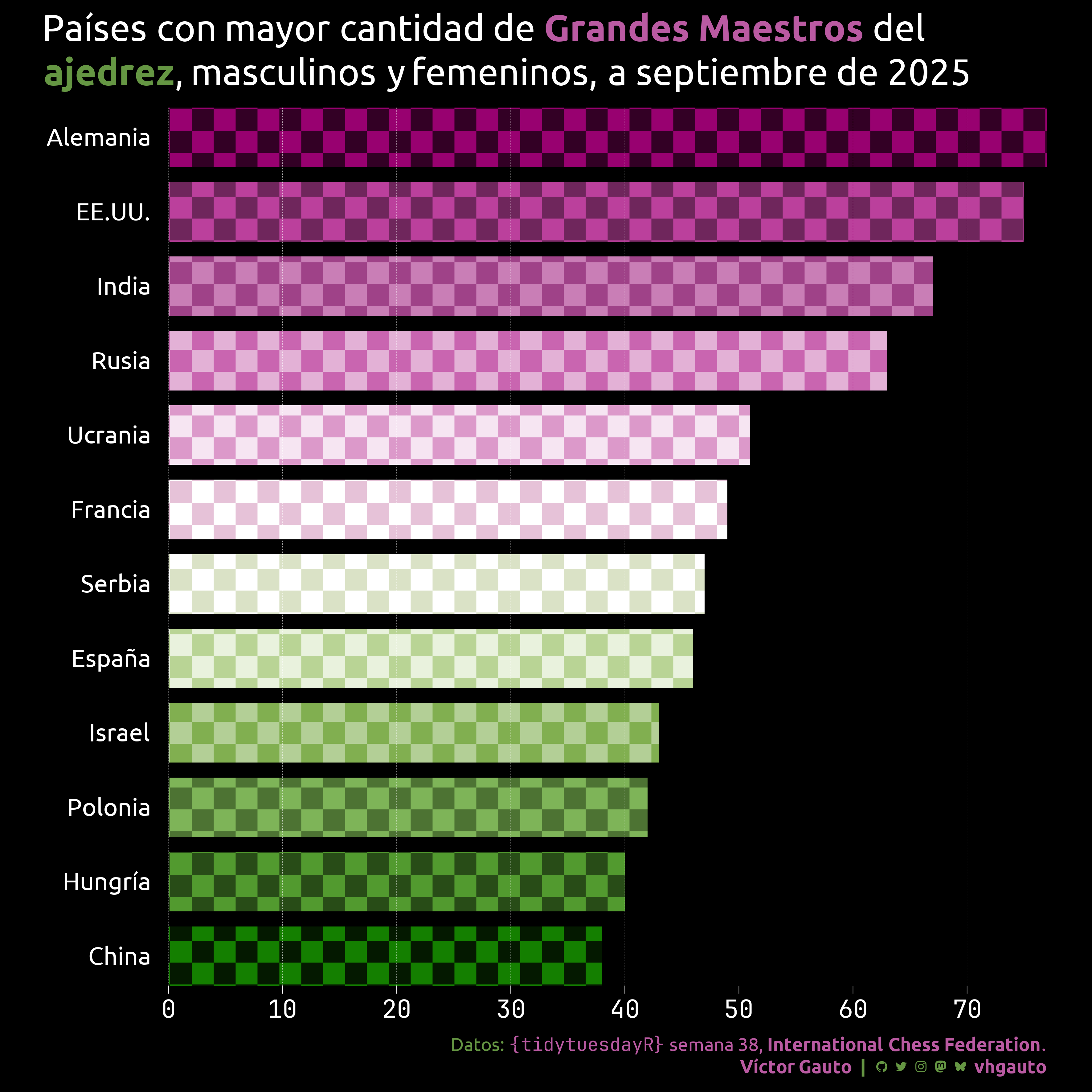
library(tidyverse)Países con la mayor cantidad de Grandes Maestros de ajedrez.
library(glue)
library(ggtext)
library(showtext)
library(grid)
library(tidyverse)Colores.
c1 <- "black"
c2 <- "white"
c3 <- "#BA5AA2"
c4 <- "#659643"
Fuentes: Ubuntu y JetBrains Mono.
font_add(
  family = "ubuntu",
  regular = "././fuente/Ubuntu-Regular.ttf",
  bold = "././fuente/Ubuntu-Bold.ttf",
  italic = "././fuente/Ubuntu-Italic.ttf"
)

font_add(
  family = "jet",
  regular = "././fuente/JetBrainsMonoNLNerdFontMono-Regular.ttf"
)

showtext_auto()
showtext_opts(dpi = 300)fuente <- glue(
"Datos: <span style='color:{c3};'><span style='font-family:jet;'>",
"{{<b>tidytuesdayR</b>}}</span> semana 38, ",
"<b>International Chess Federation</b>.</span>"
)
autor <- glue("<span style='color:{c3};'>**Víctor Gauto**</span>")
icon_twitter <- glue("<span style='font-family:jet;'></span>")
icon_instagram <- glue("<span style='font-family:jet;'></span>")
icon_github <- glue("<span style='font-family:jet;'></span>")
icon_mastodon <- glue("<span style='font-family:jet;'>󰫑</span>")
icon_bsky <- glue("<span style='font-family:jet;'></span>")
usuario <- glue("<span style='color:{c3};'>**vhgauto**</span>")
sep <- glue("**|**")
mi_caption <- glue(
"{fuente}<br>{autor} {sep} {icon_github} {icon_twitter} {icon_instagram} ",
"{icon_mastodon} {icon_bsky} {usuario}"
)tuesdata <- tidytuesdayR::tt_load(2025, 38)
september <- tuesdata$fide_ratings_septemberMe interesan los países con mayor cantidad de Grandes Maestros.
Obtengo los nombres de los países de acuerdo con la abreviatura de sus federaciones.
fed_tbl <- rvest::read_html(
  "https://www.mark-weeks.com/aboutcom/mw15b16.htm"
) |>
  rvest::html_table() |>
  pluck(2) |>
  rename_with(tolower) |>
  select(fed, country)
Selecciono septiembre de 2025 como el mes de interés y creo datos con las traducciones de los países.
d <- inner_join(september, fed_tbl, by = join_by(fed)) |>
  filter(title %in% c("GM", "FGM")) |>
  count(country, sort = TRUE) |>
  mutate(country = fct_reorder(country, n)) |>
  slice_max(order_by = country, n = 12)

country_tbl <- tibble(
  country = d$country,
  pais = c(
    "Alemania",
    "EE.UU.",
    "India",
    "Rusia",
    "Ucrania",
    "Francia",
    "Serbia",
    "España",
    "Israel",
    "Polonia",
    "Hungría",
    "China"
  )
)
Combino todos los datos.
d2 <- inner_join(country_tbl, d, by = join_by(country)) |>
mutate(pais = factor(pais, levels = rev(pais)))Defino patrones para las barras usando {grid} y diferentes intensidades de colores.
f_pattern <- function(C) {
  pattern(
    gTree(
      children = gList(
        rectGrob(
          x = c(.25, .75),
          y = c(.25, .75),
          width = .5,
          height = .5,
          gp = gpar(fill = scales::col_darker(C), col = NA)
        ),
        rectGrob(
          x = c(.25, .75),
          y = c(.75, .25),
          width = .5,
          height = .5,
          gp = gpar(fill = scales::col_lighter(C), col = NA)
        )
      )
    ),
    width = .05,
    height = .05,
    extend = "repeat"
  )
}

p <- map(
  scico::scico(n = 12, palette = "bam"),
  f_pattern
)
Título y figura.
mi_titulo <- glue(
  "Países con mayor cantidad de <b style='color: {c3};'>Grandes Maestros</b> ",
  " del<br><b style='color: {c4};'>ajedrez</b>, masculinos y femeninos, a ",
  "septiembre de 2025"
)

g <- ggplot(d2, aes(n, pais, fill = pais)) +
  geom_col(show.legend = FALSE, width = .8, fill = p) +
  scale_x_continuous(breaks = scales::breaks_width(10)) +
  coord_cartesian(expand = FALSE) +
  labs(x = NULL, y = NULL, title = mi_titulo, caption = mi_caption) +
  theme_bw(base_size = 24, base_family = "ubuntu") +
  theme(
    text = element_text(color = c2),
    aspect.ratio = 1,
    axis.ticks.y = element_blank(),
    axis.ticks.x = element_line(color = c2, linewidth = .2),
    panel.border = element_blank(),
    panel.background = element_blank(),
    panel.grid = element_blank(),
    panel.grid.major.x = element_line(
      color = c2,
      linewidth = .1,
      linetype = "55"
    ),
    panel.ontop = TRUE,
    axis.text = element_text(color = c2),
    axis.text.x = element_text(family = "jet"),
    axis.text.y = element_text(margin = margin(r = 15)),
    plot.background = element_rect(fill = c1, color = NA),
    plot.title = element_markdown(lineheight = 1.2),
    plot.title.position = "plot",
    plot.caption = element_markdown(
      size = rel(.6),
      lineheight = 1.2,
      color = c4
    )
  )
Guardo.
ggsave(
  plot = g,
  filename = "tidytuesday/2025/semana_38.png",
  width = 30,
  height = 30,
  units = "cm"
)