Ocultar código
library(glue)
library(ggtext)
library(showtext)
library(tidyterra)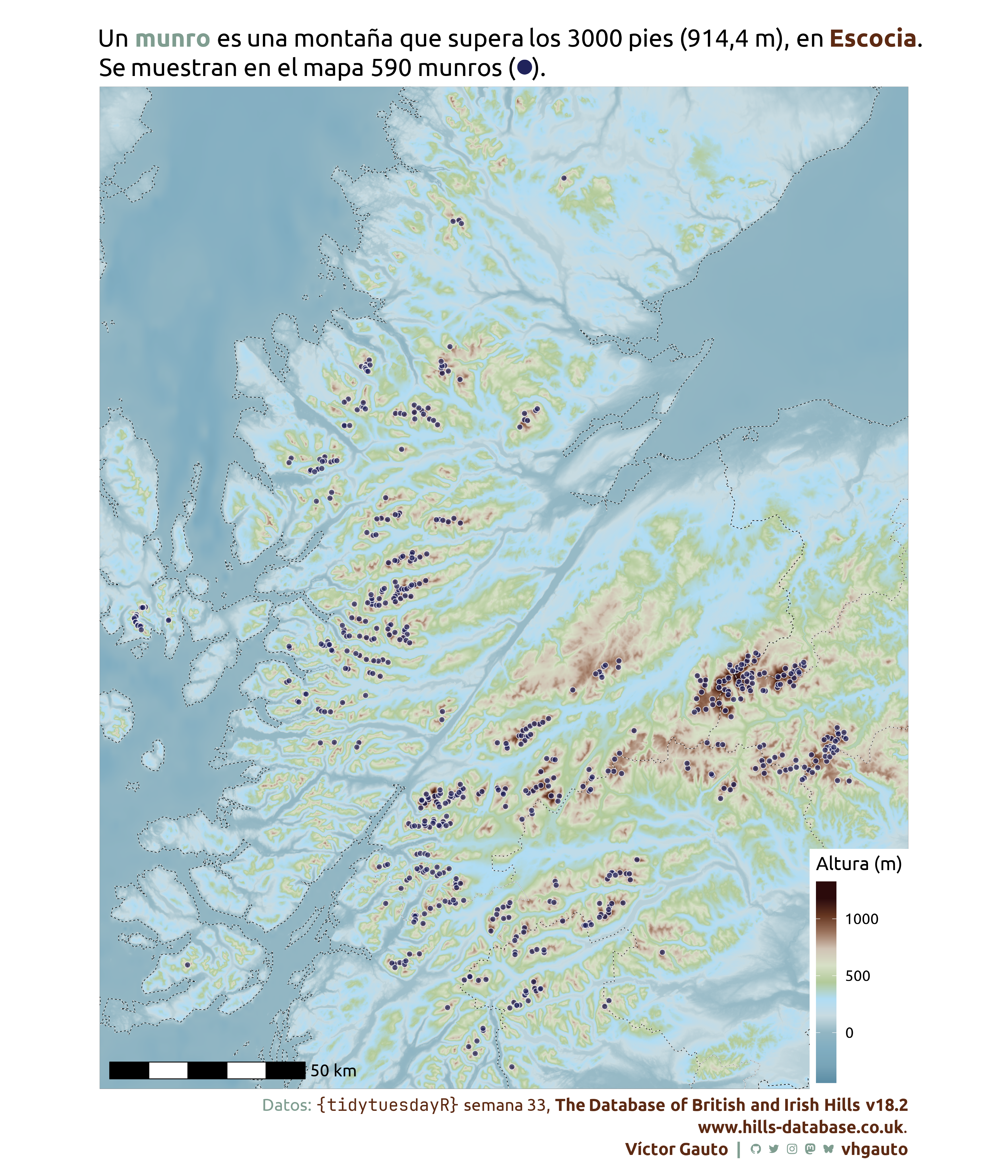
library(tidyverse)Ubicación de munros en Escocia.
library(glue)
library(ggtext)
library(showtext)
library(tidyterra)
library(tidyverse)Colores.
c1 <- "#5D2A13"
c2 <- "#7F9D90"
c3 <- "black"
c4 <- "white"
c5 <- "#20235B"
Fuentes: Ubuntu y JetBrains Mono.
font_add(
  family = "ubuntu",
  regular = "././fuente/Ubuntu-Regular.ttf",
  bold = "././fuente/Ubuntu-Bold.ttf",
  italic = "././fuente/Ubuntu-Italic.ttf"
)

font_add(
  family = "jet",
  regular = "././fuente/JetBrainsMonoNLNerdFontMono-Regular.ttf"
)

showtext_auto()
showtext_opts(dpi = 300)fuente <- glue(
"Datos: <span style='color:{c1};'><span style='font-family:jet;'>",
"{{<b>tidytuesdayR</b>}}</span> semana 33, ",
"<b>The Database of British and Irish Hills v18.2<br>www.hills-database.co.uk</b>.</span>"
)
autor <- glue("<span style='color:{c1};'>**Víctor Gauto**</span>")
icon_twitter <- glue("<span style='font-family:jet;'></span>")
icon_instagram <- glue("<span style='font-family:jet;'></span>")
icon_github <- glue("<span style='font-family:jet;'></span>")
icon_mastodon <- glue("<span style='font-family:jet;'>󰫑</span>")
icon_bsky <- glue("<span style='font-family:jet;'></span>")
usuario <- glue("<span style='color:{c1};'>**vhgauto**</span>")
sep <- glue("**|**")
mi_caption <- glue(
"{fuente}<br>{autor} {sep} {icon_github} {icon_twitter} {icon_instagram} ",
"{icon_mastodon} {icon_bsky} {usuario}"
)tuesdata <- tidytuesdayR::tt_load(2025, 33)
scottish_munros <- tuesdata$scottish_munrosMe interesa el mapa del relieve de la región indicando los munros.
Extraigo la extensión de los munros y recorto el vector de los sitios.
v <- scottish_munros |>
  select(Name, xcoord, ycoord) |>
  terra::vect(geom = c("xcoord", "ycoord"), crs = "EPSG:27700") |>
  terra::ext() |>
  terra::vect(crs = "EPSG:27700") |>
  terra::project("EPSG:4326")

p <- scottish_munros |>
  select(Name, xcoord, ycoord, Height_ft) |>
  filter(Height_ft > 3000) |>
  terra::vect(
    geom = c("xcoord", "ycoord"),
    crs = "EPSG:27700"
  ) |>
  terra::project("EPSG:4326")

p <- terra::crop(p, v)
Obtengo la elevación de la región, suavizo con una ventana de 3x3 y almaceno para una lectura posterior rápida.
e2 <- elevatr::get_elev_raster(
  locations = sf::st_as_sf(v),
  z = 10,
  clip = "bbox"
) |>
  terra::rast()

e <- terra::focal(e2, fun = median, w = 3)

terra::writeRaster(e, "tidytuesday/2025/semana_33.tif", overwrite = TRUE)
Polígono de Reino Unido, con sus divisiones administrativas.
gb <- rgeoboundaries::gb_adm2(country = "GBR") |>
terra::vect()Defino la paleta de colores, título y extensión del mapa.
col <- hypsometric_tints_db |>
filter(pal == "meyers") |>
pull(hex)
triangulo <- glue("<span style='font-family:jet; color: {c5}'>󰔶</span>")
mi_titulo <- glue(
"Un <b style='color: {c2}'>munro</b> es una montaña que supera los 3000 pies (914,4 m), en <b style='color: {c1}'>Escocia</b>.<br>Se muestran en el mapa {nrow(p)} munros ({triangulo})."
)
ext <- terra::ext(e)Mapa, con escala.
g <- ggplot() +
  geom_spatraster(
    data = e,
    maxcell = prod(dim(e))
  ) +
  geom_spatvector(
    data = gb2,
    fill = NA,
    color = c3,
    linetype = 1,
    linewidth = .2
  ) +
  geom_spatvector(
    data = esc_crop,
    fill = NA,
    color = c4,
    linetype = 2,
    linewidth = .2
  ) +
  geom_spatvector(
    data = p,
    show.legend = FALSE,
    color = c5,
    shape = 17,
    size = 2,
    alpha = .7
  ) +
  ggspatial::annotation_scale(
    location = "bl",
    pad_x = unit(.3, "cm"),
    pad_y = unit(.3, "cm"),
    height = unit(0.5, "cm"),
    text_family = "ubuntu",
    text_cex = 1.2
  ) +
  scale_fill_gradientn(
    colors = col
  ) +
  coord_sf(
    expand = FALSE,
    xlim = c(ext$xmin, ext$xmax),
    ylim = c(ext$ymin, ext$ymax)
  ) +
  labs(fill = "Altura (m)", title = mi_titulo, caption = mi_caption) +
  theme_void(base_family = "ubuntu", base_size = 16) +
  theme(
    plot.margin = margin(b = 15, t = 25),
    plot.background = element_rect(fill = "white", color = NA),
    plot.title = element_markdown(
      size = rel(1.3),
      lineheight = 1.2,
      margin = margin(b = 5)
    ),
    plot.caption = element_markdown(
      color = c2,
      lineheight = 1.3,
      size = rel(.9)
    ),
    legend.position = "inside",
    legend.background = element_rect(fill = "white", color = "white"),
    legend.justification.inside = c(1, 0),
    legend.key.height = unit(1.2, "cm"),
    legend.margin = margin(5, 5, 5, 5)
  )
Guardo.
ggsave(
  plot = g,
  filename = "tidytuesday/2025/semana_33.png",
  width = 30,
  height = 35,
  units = "cm"
)