# paquetes ----------------------------------------------------------------
library(tidyverse)
library(patchwork)
library(ggtext)
library(showtext)
library(ggpath)
library(glue)
# fuentes -----------------------------------------------------------------
fondo <- "#2e233c"
col1 <- "#b86092"
col2 <- "#df9ed4"
col3 <- "#574571"
# título
font_add_google(name = "Bonheur Royale", family = "royale", db_cache = FALSE)
# subtítulo
font_add_google(name = "Anuphan", family = "anuphan", db_cache = FALSE)
# texto vertical
font_add_google(name = "Cutive Mono", family = "cutive", db_cache = FALSE)
# texto horizontal
font_add_google(name = "Bebas Neue", family = "bebas", db_cache = FALSE)
showtext_auto()
showtext_opts(dpi = 300)
# íconos
font_add("fa-reg", "icon/Font Awesome 6 Free-Regular-400.otf")
font_add("fa-brands", "icon/Font Awesome 6 Brands-Regular-400.otf")
font_add("fa-solid", "icon/Font Awesome 6 Free-Solid-900.otf")
showtext_auto()
showtext_opts(dpi = 300)
# caption
fuente <- glue("Datos: <span style='color:{col2};'><span style='font-family:mono;'>{{<b>tidytuesdayR</b>}}</span> semana 17</span>")
autor <- glue("Autor: <span style='color:{col2};'>**Víctor Gauto**</span>")
icon_twitter <- glue("<span style='font-family:fa-brands;'></span>")
icon_github <- glue("<span style='font-family:fa-brands;'></span>")
usuario <- glue("<span style='color:{col2};'>**vhgauto**</span>")
sep <- glue("**|**")
mi_caption <- glue("{fuente} {sep} {autor} {sep} {icon_github} {icon_twitter} {usuario}")
# ícono de correr
correr <- "<span style='font-family:fa-solid;'></span>"
# datos -------------------------------------------------------------------
browseURL("https://github.com/rfordatascience/tidytuesday/blob/master/data/2023/2023-04-25/readme.md")
winners <- readr::read_csv('https://raw.githubusercontent.com/rfordatascience/tidytuesday/master/data/2023/2023-04-25/winners.csv') |>
janitor::clean_names()
london_marathon <- readr::read_csv('https://raw.githubusercontent.com/rfordatascience/tidytuesday/master/data/2023/2023-04-25/london_marathon.csv') |>
janitor::clean_names()
# arreglo de los datos
# me interesa la relación entre los que inician la maratón y los que la terminan
datos <- london_marathon |>
drop_na(finishers, starters) |>
mutate(rel = finishers/starters*100) |>
filter(rel > 80) |>
mutate(año = year(date)) |>
mutate(icon = correr)
# figura ------------------------------------------------------------------
# texto subtítulo
subtitulo <- tibble(
año = 1995,
rel = 93,
label = glue(
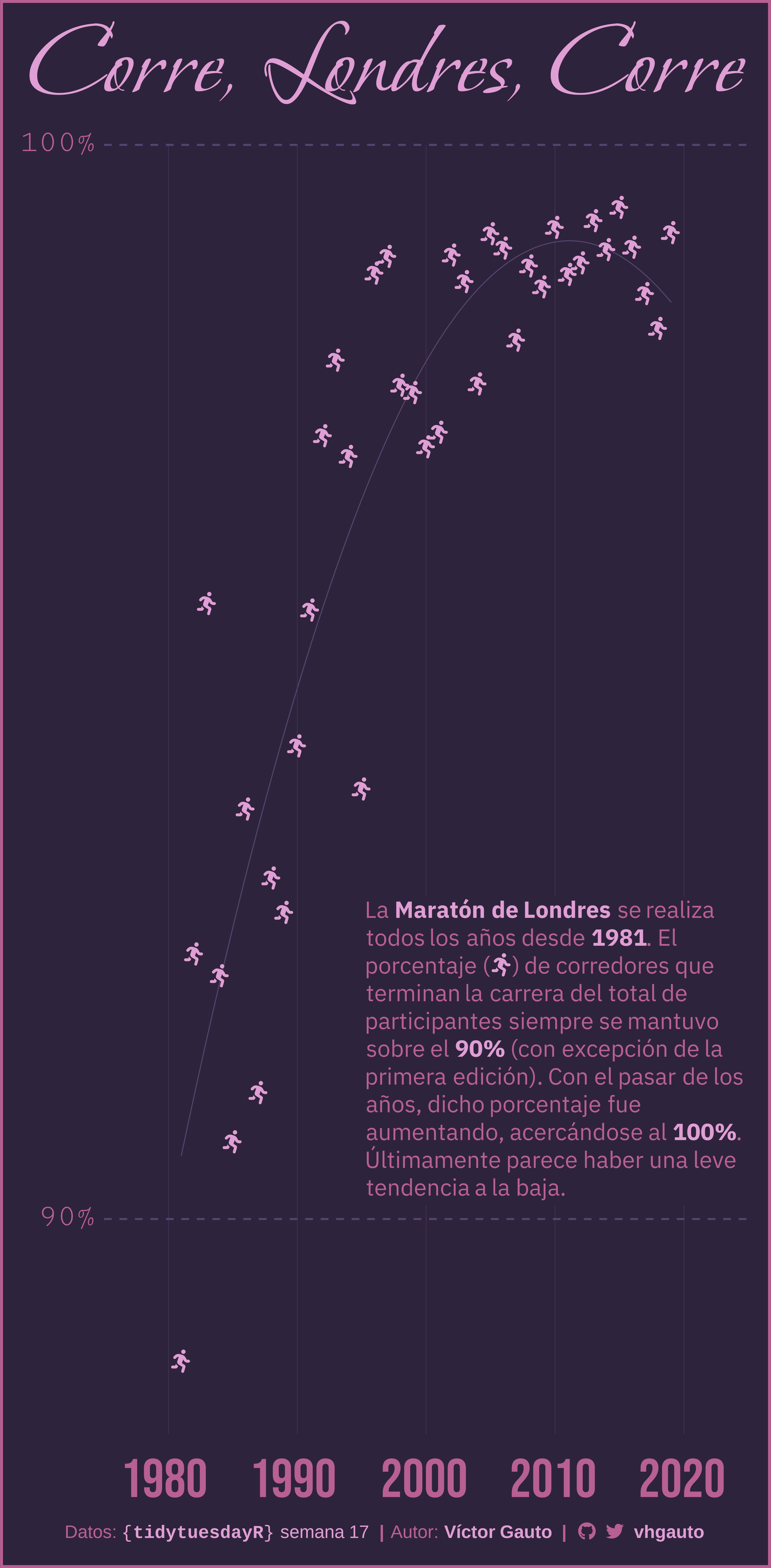
"La <span style='color:{col2};'>**Maratón de Londres**</span> se realiza todos
los años desde <span style='color:{col2};'>**{min(datos$año)}**</span>. El
porcentaje (<span style='color:{col2};'>**{correr}**</span>) de corredores
que terminan la carrera del total de participantes siempre se mantuvo sobre
el <span style='color:{col2};'>**90%**</span> (con excepción de la primera
edición). Con el pasar de los años, dicho porcentaje fue aumentando,
acercándose al <span style='color:{col2};'>**100%**</span>. Últimamente
parece haber una leve tendencia a la baja."))
# figura
g1 <- datos |>
ggplot(aes(x = año, y = rel)) +
# líneas verticales
geom_vline(
xintercept = seq(1980, 2020, 10), color = col3, linewidth = .15) +
# líneas horizontales
geom_hline(
yintercept = c(90, 100), color = col3, linewidth = 1, linetype = 2) +
# tendencia
geom_smooth(
method = "loess", formula = y ~ x, span = 2, color = col3, linewidth = .5,
se = FALSE, linetype = 1, lineend = "round") +
# puntos
geom_richtext(
aes(label = icon), color = col2, label.color = NA, fill = NA, size = 9) +
# subtítulos
geom_textbox(
data = subtitulo, aes(label = label), box.color = NA, fill = fondo, size = 9,
color = col1, hjust = 0, vjust = 1, family = "anuphan",
width = unit(6, "inch")) +
# ejes
scale_x_continuous(
breaks = c(1975, seq(1980, 2020, 10), 2025),
labels = c("", seq(1980, 2020, 10), ""),
limits = c(1975, 2025),
expand = c(0, 0)) +
scale_y_continuous(
breaks = c(90, 100),
limits = c(88, 100),
labels = scales::label_number(
big.mark = ".", decimal.mark = ",", suffix = "%"),
expand = c(0, 0)) +
coord_cartesian(clip = "off") +
labs(title = "Corre, Londres, Corre", x = NULL, y = NULL, caption = mi_caption) +
# temas
theme_minimal() +
theme(
aspect.ratio = 2,
plot.margin = margin(14, 25, 29, 25),
plot.background = element_rect(
fill = fondo, color = col1, linewidth = 3),
plot.title.position = "plot",
plot.title = element_markdown(
size = 120, color = col2, family = "royale", hjust = .5,
margin = margin(10, 0, 20, 0)),
plot.caption = element_markdown(
color = col1, size = 20, hjust = -6.6, margin = margin(25, 0, 0, 0)),
axis.text = element_markdown(color = col1),
axis.text.x = element_markdown(
margin = margin(25, 0, 0, 0), family = "bebas", size = 60),
axis.text.y = element_markdown(vjust = .5, family = "cutive", size = 35),
panel.grid = element_blank()
)
# guardo
ggsave(
plot = g1,
filename = "2023/semana_17/viz.png",
width = 30,
height = 61,
units = "cm",
dpi = 300)
# abro
browseURL("2023/semana_17/viz.png")