Ocultar código
library(glue)
library(ggtext)
library(showtext)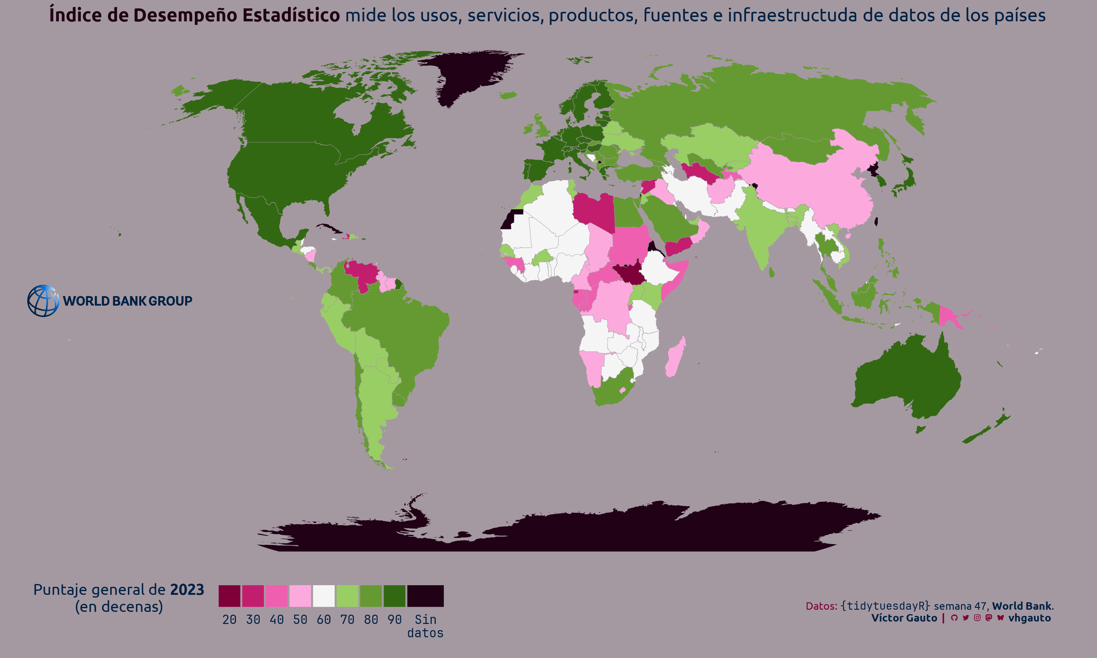
library(tidyverse)Índice de desempeño estadístico por país en 2023.
library(glue)
library(ggtext)
library(showtext)
library(tidyverse)Colores.
c1 <- "#a599a1"
c2 <- "#002244"
c3 <- "#7f0038"
c4 <- "#200116"
Fuentes: Ubuntu y JetBrains Mono.
font_add(
  family = "ubuntu",
  regular = "././fuente/Ubuntu-Regular.ttf",
  bold = "././fuente/Ubuntu-Bold.ttf",
  italic = "././fuente/Ubuntu-Italic.ttf"
)

font_add(
  family = "jet",
  regular = "././fuente/JetBrainsMonoNLNerdFontMono-Regular.ttf"
)

showtext_auto()
showtext_opts(dpi = 300)fuente <- glue(
"Datos: <span style='color:{c2};'><span style='font-family:jet;'>",
"{{<b>tidytuesdayR</b>}}</span> semana 47, ",
"<b>World Bank</b>.</span>"
)
autor <- glue("<span style='color:{c2};'>**Víctor Gauto**</span>")
icon_twitter <- glue("<span style='font-family:jet;'></span>")
icon_instagram <- glue("<span style='font-family:jet;'></span>")
icon_github <- glue("<span style='font-family:jet;'></span>")
icon_mastodon <- glue("<span style='font-family:jet;'>󰫑</span>")
icon_bsky <- glue("<span style='font-family:jet;'></span>")
usuario <- glue("<span style='color:{c2};'>**vhgauto**</span>")
sep <- glue("**|**")
mi_caption <- glue(
"{fuente}<br>{autor} {sep} {icon_github} {icon_twitter} {icon_instagram} ",
"{icon_mastodon} {icon_bsky} {usuario}"
)tuesdata <- tidytuesdayR::tt_load(2025, 47)
spi_indicators <- tuesdata$spi_indicatorsMe interesa el índice general de desempeño estadístico mostrado en un mapa.
Obtengo vector de todos los países.
mundo <- rgeoboundaries::gb_adm0() |>
  rename(iso3c = shapeGroup)
Filtro los datos al año 2023 y calculo la decena del puntaje general.
d <- filter(spi_indicators, year == 2023) |>
  select(iso3c, overall_score) |>
  drop_na() |>
  mutate(rango = overall_score - overall_score %% 10) |>
  mutate(rango = factor(rango))
Combino los datos con el vector países. Agrego una nueva categoría al rando de puntaje para incluir los países son datos.
d_mundo <- full_join(d, mundo, by = join_by(iso3c)) |>
  sf::st_as_sf() |>
  sf::st_transform("ESRI:54030") |>
mutate(rango = if_else(is.na(rango), factor("Sin\ndatos"), rango))Logo del Banco Mundial y título.
img_tbl <- tibble(
  x = I(.1),
  y = I(.5),
  image = "https://upload.wikimedia.org/wikipedia/commons/thumb/c/ca/World_Bank_Group_logo.svg/1280px-World_Bank_Group_logo.svg.png"
)

mi_titulo <- glue(
  "<b style='color: {c4}'>Índice de Desempeño Estadístico</b> mide los usos, ",
  "servicios, productos, fuentes e infraestructuda de datos de los países"
)
Figura.
g <- ggplot() +
  tidyterra::geom_spatvector(
    data = d_mundo,
    aes(fill = rango),
    color = c1,
    linewidth = .1
  ) +
  ggimage::geom_image(
    data = img_tbl,
    aes(x, y, image = image),
    inherit.aes = FALSE,
    size = .3
  ) +
  scale_fill_manual(
    breaks = c(seq(20, 90, 10), "Sin\ndatos"),
    labels = c(seq(20, 90, 10), "Sin\ndatos"),
    values = c(PrettyCols::prettycols(palette = "PinkGreens", n = 8), c4)
  ) +
  labs(
    title = mi_titulo,
    fill = "Puntaje general de **2023**<br>(en decenas)",
    caption = mi_caption
  ) +
  guides(fill = guide_legend(nrow = 1)) +
  theme_void(base_size = 12, base_family = "ubuntu") +
  theme_sub_plot(
    background = element_rect(fill = c1),
    title = element_markdown(color = c2, hjust = .5),
    caption = element_markdown(
      color = c3,
      hjust = .95,
      size = rel(.7),
      lineheight = 1.1,
      margin = margin(t = -30)
    )
  ) +
  theme_sub_legend(
    position = "bottom",
    justification.bottom = .05,
    title = element_markdown(
      color = c2,
      margin = margin(b = 20, r = 10),
      lineheight = 1.1,
      hjust = .5
    ),
    text = element_text(color = c2, family = "jet"),
    text.position = "bottom",
    key.spacing.x = unit(1, "pt")
  )
Guardo.
ggsave(
  plot = g,
  filename = "tidytuesday/2025/semana_47.png",
  width = 30,
  height = 18,
  units = "cm"
)