Ocultar código
library(glue)
library(ggtext)
library(showtext)
library(patchwork)
library(tidyterra)
library(tidyverse)Ubicaciones de ranas en Australia.
library(glue)
library(ggtext)
library(showtext)
library(patchwork)
library(tidyterra)
library(tidyverse)Colores.
c1 <- "#AD8CAE"
c2 <- "#BF616A"
c3 <- "grey95"
c4 <- "#485D32"
Fuentes: Ubuntu y JetBrains Mono.
font_add(
  family = "ubuntu",
  regular = "././fuente/Ubuntu-Regular.ttf",
  bold = "././fuente/Ubuntu-Bold.ttf",
  italic = "././fuente/Ubuntu-Italic.ttf"
)

font_add(
  family = "jet",
  regular = "././fuente/JetBrainsMonoNLNerdFontMono-Regular.ttf"
)

showtext_auto()
showtext_opts(dpi = 300)fuente <- glue(
"Datos: <span style='color:{c1};'><span style='font-family:jet;'>",
"{{<b>tidytuesdayR</b>}}</span> semana 35, ",
"<b>FrogID</b>.</span>"
)
autor <- glue("<span style='color:{c1};'>**Víctor Gauto**</span>")
icon_twitter <- glue("<span style='font-family:jet;'></span>")
icon_instagram <- glue("<span style='font-family:jet;'></span>")
icon_github <- glue("<span style='font-family:jet;'></span>")
icon_mastodon <- glue("<span style='font-family:jet;'>󰫑</span>")
icon_bsky <- glue("<span style='font-family:jet;'></span>")
usuario <- glue("<span style='color:{c1};'>**vhgauto**</span>")
sep <- glue("**|**")
mi_caption <- glue(
"{fuente}<br>{autor} {sep} {icon_github} {icon_twitter} {icon_instagram} ",
"{icon_mastodon} {icon_bsky} {usuario}"
)tuesdata <- tidytuesdayR::tt_load(2025, 35)
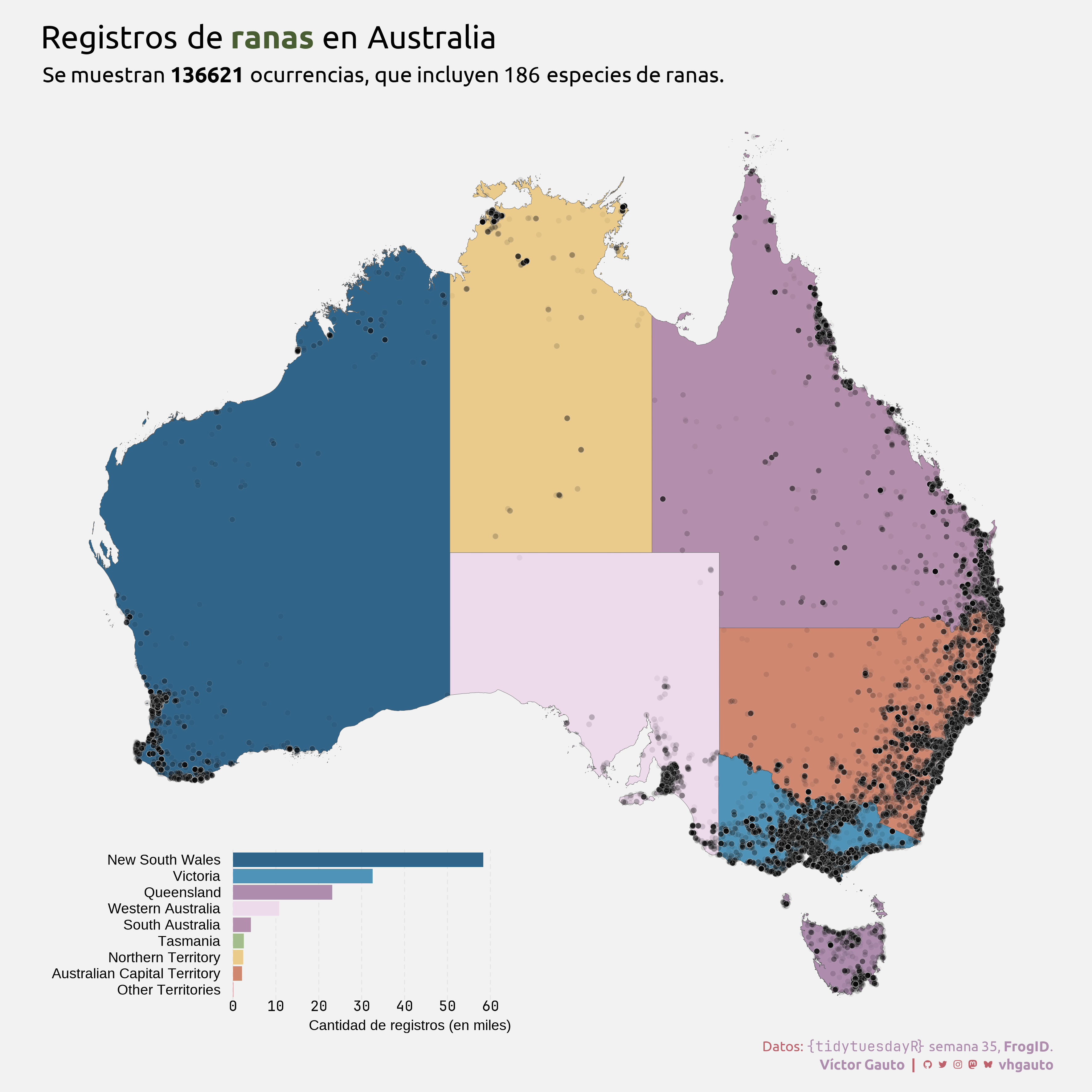
frogID_data <- tuesdata$frogID_dataMe interesa ver un mapa de las posiciones de las ranas registradas y la cantidad de registros por división de Australia.
Creo vector de puntos.
v <- frogID_data |>
  terra::vect(
    geom = c("decimalLongitude", "decimalLatitude"),
    crs = "EPSG:4326"
  )
Obtengo vector de Australia y recorto la extensión.
aus <- rgeoboundaries::gb_adm1(country = "AUS") |>
  terra::vect()

aus_ext <- terra::ext(aus)
aus_ext2 <- terra::ext(112, 156, aus_ext$ymin, aus_ext$ymax) |>
  terra::vect(crs = "EPSG:4326")

aus2 <- terra::crop(aus, aus_ext2)

v2 <- sf::st_intersection(sf::st_as_sf(v), sf::st_as_sf(aus2))
Cuento la cantidad por estado.
d <- count(v2, shapeName) |>
  sf::st_drop_geometry() |>
mutate(shapeName = fct_reorder(shapeName, n))Título y subtítulo.
mi_titulo <- glue(
  "Registros de <b style='color: {c4}'>ranas</b> en Australia"
)

mi_subitulo <- glue(
  "Se muestran **{nrow(frogID_data)}** ocurrencias, que incluyen {length(unique(frogID_data$scientificName))} especies de ranas."
)
Figura de columnas.
g_col <- ggplot(d, aes(n, shapeName, fill = shapeName)) +
  geom_col(show.legend = FALSE) +
  scale_fill_manual(
    values = alpha(
      c(nord::nord(palette = "aurora"), nord::nord(palette = "lumina")),
      1
    )
  ) +
  scale_x_continuous(
    labels = scales::label_number(
      big.mark = ".",
      decimal.mark = ",",
      scale = 1e-3
    ),
    breaks = scales::breaks_width(1e4)
  ) +
  coord_cartesian(clip = "off") +
  labs(x = "Cantidad de registros (en miles)", y = NULL) +
  theme_void() +
  theme(
    plot.background = element_rect(fill = "grey95", color = NA),
    panel.grid.major.x = element_line(color = "grey90", linetype = 2),
    legend.position = "none",
    axis.text.x = element_text(family = "jet"),
    axis.text.y = element_text(hjust = 1),
    axis.title.x = element_text(hjust = 1.2, margin = margin(t = 5))
  )
Mapa de Australia con los puntos.
g <- ggplot() +
  geom_spatvector(
    data = aus2,
    aes(fill = shapeName),
    linewidth = .1
  ) +
  geom_spatvector(
    data = v2,
    alpha = 1 / 20,
    size = 2,
    color = "white",
    fill = "black",
    stroke = .2,
    shape = 21
  ) +
  scale_fill_manual(
    values = alpha(
      c(nord::nord(palette = "aurora"), nord::nord(palette = "lumina")),
      1
    )
  ) +
  theme_void(base_size = 5, base_family = "ubuntu") +
  theme(
    legend.position = "none"
  )
Figura compuesta.
g_comp <- g +
  inset_element(
    g_col,
    left = .01,
    bottom = .01,
    right = .45,
    top = .2
  ) +
  plot_annotation(
    title = mi_titulo,
    subtitle = mi_subitulo,
    caption = mi_caption,
    theme = theme(
      plot.background = element_rect(fill = NA, color = NA),
      plot.title = element_markdown(
        family = "ubuntu",
        size = 25,
        margin = margin(t = 15)
      ),
      plot.subtitle = element_markdown(
        family = "ubuntu",
        size = 17,
        margin = margin(t = 10)
      ),
      plot.caption = element_markdown(
        family = "ubuntu",
        color = c2,
        size = 11,
        lineheight = 1.3,
        margin = margin(b = 10, r = -4)
      )
    )
  )
Guardo.
ggsave(
  plot = g_comp,
  filename = "tidytuesday/2025/semana_35.png",
  width = 30,
  height = 30,
  units = "cm"
)