Ocultar código
library(glue)
library(ggtext)
library(showtext)
library(tidyverse)Tendencias de accidentes fatales diarios en EE.UU, entre 1992 y 2016
library(glue)
library(ggtext)
library(showtext)
library(tidyverse)Colores.
col <- monochromeR::generate_palette(
  "#704D9E", modification = "go_both_ways", n_colours = 6
)
Fuentes: Ubuntu y JetBrains Mono.
font_add(
  family = "ubuntu",
  regular = "././fuente/Ubuntu-Regular.ttf",
  bold = "././fuente/Ubuntu-Bold.ttf",
  italic = "././fuente/Ubuntu-Italic.ttf"
)

font_add(
  family = "jet",
  regular = "././fuente/JetBrainsMonoNLNerdFontMono-Regular.ttf"
)

showtext_auto()
showtext_opts(dpi = 300)fuente <- glue(
"Datos: <span style='color:{col[6]};'><span style='font-family:jet;'>",
"{{<b>tidytuesdayR</b>}}</span> semana 16, ",
"<b>The annual cannabis holiday and fatal traffic crashes<br></b>
S. Harper, A. Palayew.</span>"
)
autor <- glue("<span style='color:{col[6]};'>**Víctor Gauto**</span>")
icon_twitter <- glue("<span style='font-family:jet;'></span>")
icon_instagram <- glue("<span style='font-family:jet;'></span>")
icon_github <- glue("<span style='font-family:jet;'></span>")
icon_mastodon <- glue("<span style='font-family:jet;'>󰫑</span>")
icon_bsky <- glue("<span style='font-family:jet;'></span>")
usuario <- glue("<span style='color:{col[6]};'>**vhgauto**</span>")
sep <- glue("**|**")
mi_caption <- glue(
"{fuente}<br>{autor} {sep} {icon_github} {icon_twitter} {icon_instagram} ",
"{icon_mastodon} {icon_bsky} {usuario}"
)tuesdata <- tidytuesdayR::tt_load(2025, 16)
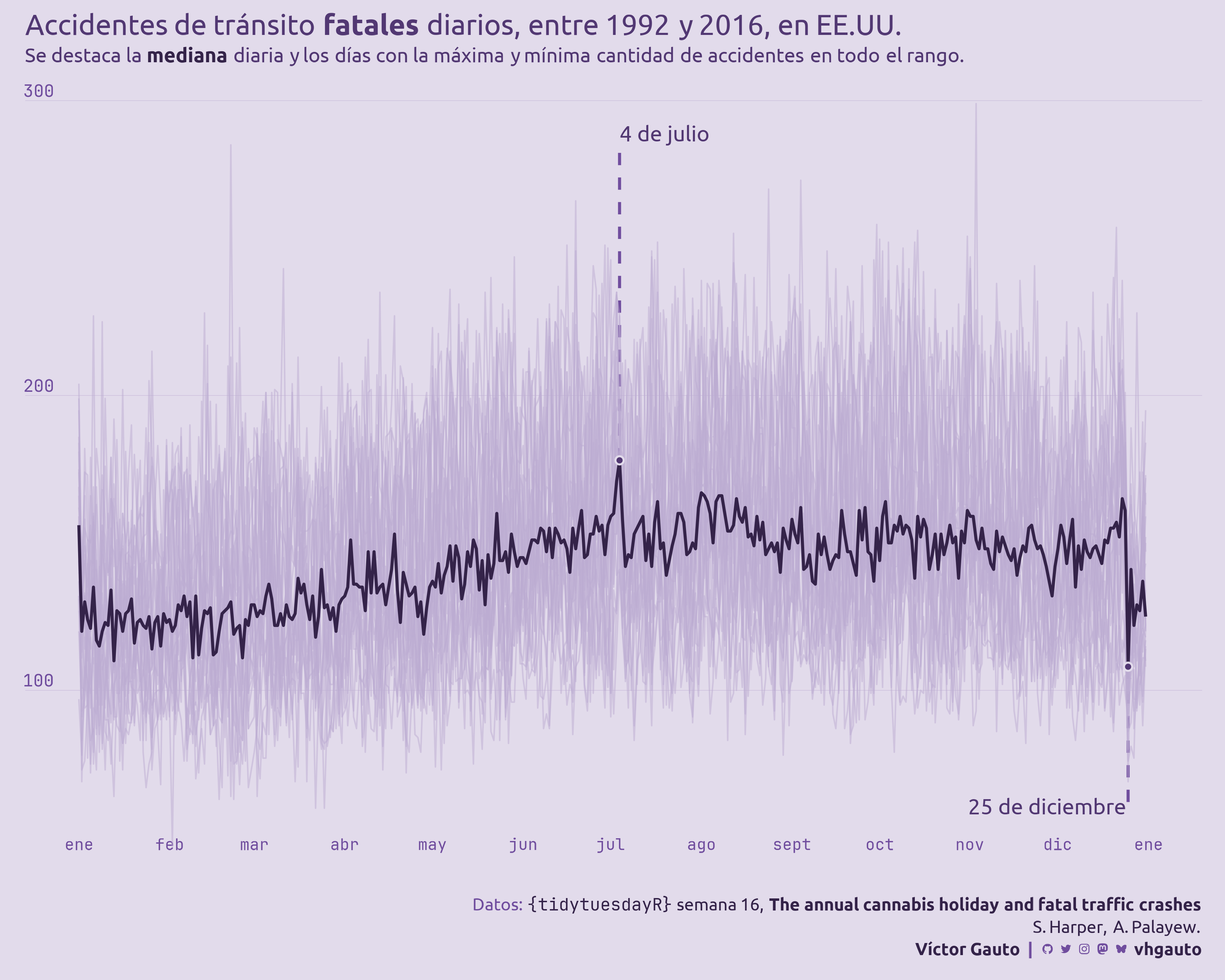
daily_accidents <- tuesdata$daily_accidentsMe interesa visualizar todos los años (d) y mostrar la mediana (d_m), con el día con la máxima cantidad de accidentes (d_max).
d <- daily_accidents |>
  mutate(
    fecha = make_date(year = 2020, month = month(date), day = day(date)),
    año = year(date),
    dia = yday(date)
  ) |>
  arrange(dia, date)

d_m <- d |>
  reframe(
    m = median(fatalities_count),
    .by = fecha
  )

d_max <- slice_max(d_m, order_by = m, n = 1)
d_min <- slice_min(d_m, order_by = m, n = 1)Etiquetas para el eje horizontal.
eje_x <- seq.Date(
  from = ymd(20200101),
  to = ymd(20210101),
  by = "1 month"
)
Título y subtítulo.
mi_titulo <- glue(
  "Accidentes de tránsito **fatales** diarios, entre 1992 y 2016, en EE.UU."
)

mi_subtitulo <- glue(
  "Se destaca la <b style='color:{col[6]}'>mediana</b> diaria y los días
  con la máxima y mínima cantidad de accidentes en todo el rango."
)
Figura.
g <- ggplot(d, aes(fecha, fatalities_count, group = year(date))) +
  annotate(
    geom = "text", x = eje_x, y = 45, label = format(eje_x, "%b"),
    vjust = -.2, color = col[4], family = "jet"
  ) +
  geom_segment(
    data = d_max,
    aes(x = fecha, y = m, yend = .95*max(d$fatalities_count), xend = fecha),
    inherit.aes = FALSE, color = col[4], linewidth = 1, linetype = 2
  ) +
  geom_segment(
    data = d_min,
    aes(x = fecha, y = m, yend = 1.25*min(d$fatalities_count), xend = fecha),
    inherit.aes = FALSE, color = col[4], linewidth = 1, linetype = 2
  ) +
  annotate(
    geom = "text", x = d_max$fecha, y = .952*max(d$fatalities_count),
    label = "4 de julio", hjust = 0, color = col[5], size = 15,
    size.unit = "pt", vjust = -.3, family = "ubuntu"
  ) +
  annotate(
    geom = "text", x = d_min$fecha-1, y = 1.2*min(d$fatalities_count),
    label = "25 de diciembre", hjust = 1, color = col[5], size = 15,
    size.unit = "pt", vjust = -.3, family = "ubuntu"
  ) +
  geom_line(alpha = .5, color = col[2]) +
  geom_line(
    data = d_m, aes(fecha, m), alpha = 1, color = col[6], linewidth = 1,
    inherit.aes = FALSE
  ) +
  geom_point(
    data = bind_rows(d_max, d_min), aes(fecha, m), size = 2, color = col[1],
    shape = 21, stroke = 1, fill = col[5], inherit.aes = FALSE
  ) +
  coord_cartesian(clip = "off") +
  labs(title = mi_titulo, subtitle = mi_subtitulo, caption = mi_caption) +
  theme_void() +
  theme(
    aspect.ratio = .7,
    text = element_text(family = "ubuntu"),
    plot.margin = margin(b = 15, r = 10, l = 10, t = 5),
    plot.background = element_rect(fill = col[1], color = NA),
    plot.title = element_markdown(size = 20, color = col[5]),
    plot.subtitle = element_markdown(size = 14, color = col[5]),
    plot.caption = element_markdown(color = col[4], lineheight = 1.3, size = 12),
    panel.grid.major.y = element_line(color = col[2], linewidth = .1),
    axis.text.y = element_text(
      margin = margin(r = -20), vjust = -.3, family = "jet", size = 12,
      color = col[4]
    )
  )

ggsave(
  plot = g,
  filename = "tidytuesday/2025/semana_16.png",
  width = 30,
  height = 24,
  units = "cm"
)

browseURL(paste0(getwd(), "/tidytuesday/2025/semana_16.png"))
Guardo.
ggsave(
  plot = g,
  filename = "tidytuesday/2025/semana_16.png",
  width = 30,
  height = 24,
  units = "cm"
)