Semana 23

Figura semana 23
geom_textpath
geom_richtext
geom_textbox
argentina
Autor
Víctor Gauto
Fecha de publicación
11 de junio de 2023
Consumo energético argentino, y su comparación con los valores medios mundiales. En combustibles fósiles y renovables.
Script

Código
# paquetes ----------------------------------------------------------------

library(tidyverse)
library(geomtextpath)
library(glue)
library(showtext)
library(ggtext)

# fuentes -----------------------------------------------------------------

# colores
c1 <- "#183471"
c2 <- "#43429B"
c3 <- "#DF9ED4"
c4 <- "#EACC62"
c5 <- "#7EC5F4"
c6 <- "#FFCD11"
c7 <- "grey90"

# años, eje horizontal
font_add_google(name = "Bebas Neue", family = "bebas", db_cache = TRUE)
# eje vertical
font_add_google(name = "Inconsolata", family = "inconsolata", db_cache = FALSE)
# resto del texto
font_add_google(name = "Ubuntu", family = "ubuntu", db_cache = FALSE)
# título
font_add_google(name = "Yeseva One", family = "yeseva", db_cache = FALSE)

showtext_auto()
showtext_opts(dpi = 300)

# íconos
font_add("fa-brands", "icon/Font Awesome 6 Brands-Regular-400.otf")

# caption
fuente <- glue("Datos: <span style='color:{c3};'><span style='font-family:mono;'>{{<b>tidytuesdayR</b>}}</span> semana 23</span>")
autor <- glue("Autor: <span style='color:{c3};'>**Víctor Gauto**</span>")
icon_twitter <- glue("<span style='font-family:fa-brands;'>&#xf099;</span>")
icon_github <- glue("<span style='font-family:fa-brands;'>&#xf09b;</span>")
usuario <- glue("<span style='color:{c3};'>**vhgauto**</span>")
sep <- glue("**|**")

mi_caption <- glue("{fuente} {sep} {autor} {sep} {icon_github} {icon_twitter} {usuario}")

# datos -------------------------------------------------------------------

browseURL("https://github.com/rfordatascience/tidytuesday/blob/master/data/2023/2023-06-06/readme.md")

energia <- readr::read_csv('https://raw.githubusercontent.com/rfordatascience/tidytuesday/master/data/2023/2023-06-06/owid-energy.csv')

# limpio los datos, enfocándome en el mundo y Argentina, renovable y fósiles
d <- energia |> 
  # filtro por Argentina y el mundo
  filter(country %in% c("Argentina", "World")) |> 
  # selecciono energías renovables y fósiles
  select(year, country, renewables_energy_per_capita, fossil_energy_per_capita) |> 
  # tabla larga
  pivot_longer(cols = -c(year, country)) |> 
  # remuevo NA
  drop_na(value) |> 
  # acomodo los nombres
  mutate(name = str_remove(name, "_energy_per_capita")) |>
  mutate(name = str_replace(name, "_", " ")) |>
  # traduzco
  mutate(country = case_match(country, "World" ~ "Mundo", .default = country)) |> 
  # agrego justificación horizontal p/usar en la figura (geom_textpath)
  mutate(hjust = case_when(
    country == "Argentina" & name == "fossil" ~ .9,
    country == "Argentina" & name == "renewables" ~ .3,
    country == "Mundo" & name == "fossil" ~ .42,
    country == "Mundo" & name == "renewables" ~ .01))

# figura ------------------------------------------------------------------

# {geomtextpath} 
browseURL("https://github.com/AllanCameron/geomtextpath")

# título
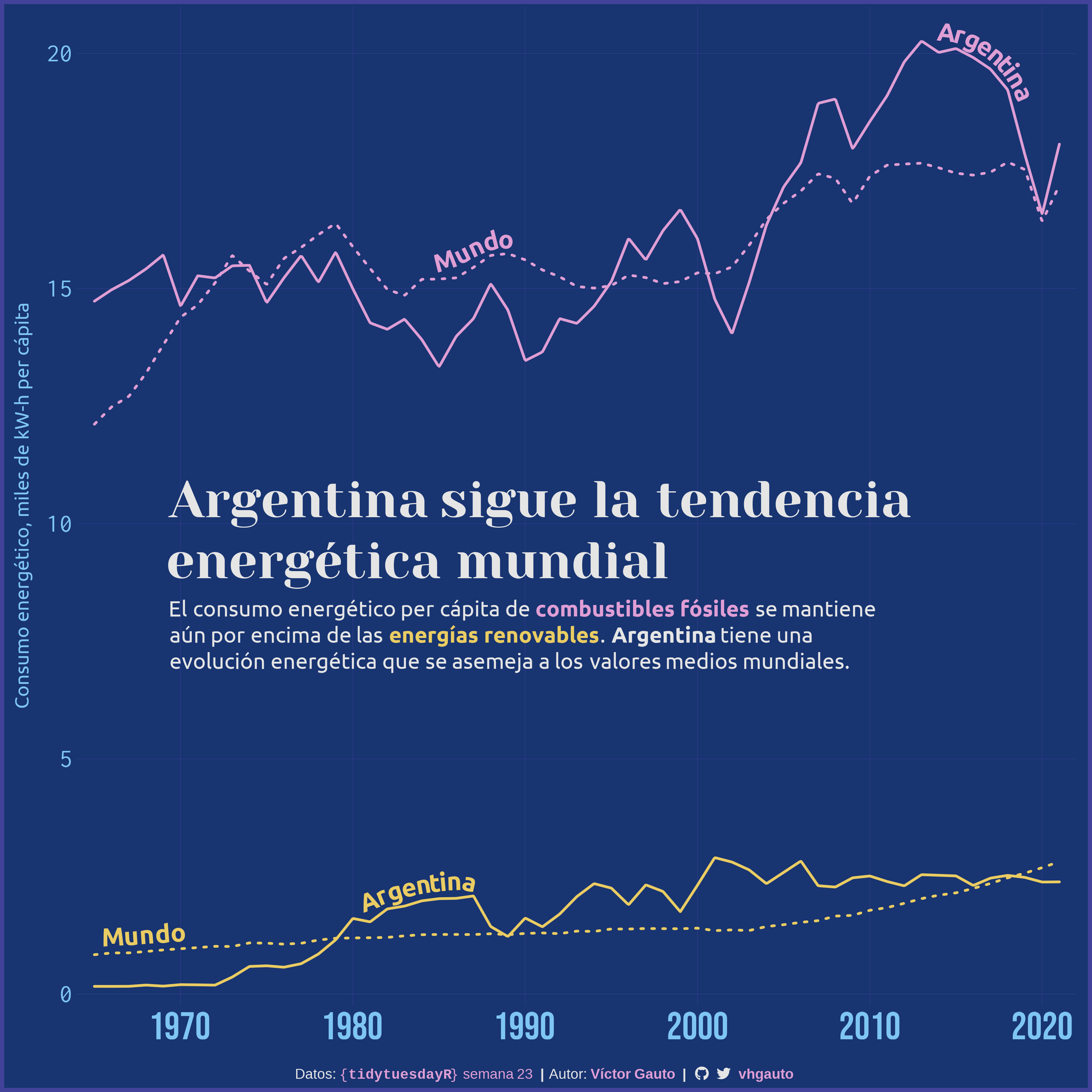
ti <- tibble(
  year = 1969,
  value = 11000,
  label = "Argentina sigue la tendencia<br>energética mundial")

# subtítulo
su <- tibble(
  year = 1969,
  value = 8500,
  label = glue(
    "El consumo energético per cápita de <b style='color:{c3};'>combustibles fósiles</b>
    se mantiene aún por encima de las <b style='color:{c4};'>energías renovables</b>. 
    **Argentina** tiene una evolución energética que se asemeja a los valores 
    medios mundiales."))

# figura
g <- ggplot(data = d, aes(x = year, y = value, color = name, linetype = country)) +
  # líneas y texto
  geom_textpath(
    aes(label = glue("**{country}**"), hjust = I(hjust)),
    vjust = -0.2, show.legend = FALSE, text_smoothing = 30, family = "ubuntu",
    size = 7, linewidth = 1, rich = TRUE, lineend = "round") +
  # título
  geom_richtext(
    data = ti, aes(x = year, y = value, label = label), inherit.aes = FALSE,
    fill = NA, label.color = NA, color = c7, size = 14, show.legend = FALSE,
    hjust = 0, vjust = 1, family = "yeseva") +
  # subtítulo
  geom_textbox(
    data = su, aes(x = year, y = value, label = label), inherit.aes = FALSE,
    fill = NA, box.color = NA, color = c7, size = 6, show.legend = FALSE,
    hjust = 0, vjust = 1, family = "ubuntu", width = unit(20, "cm")) +
  # ejes
  scale_x_continuous(
    breaks = seq(1960, 2021, 10), limits = c(1965, 2021), expand = c(0, 1)) +
  scale_y_continuous(
    breaks = seq(0, 20e3, 5e3), limits = c(-250, 21e3), expand = c(0, 0),
    labels = scales::label_number(scale = .001)) +
  scale_color_manual(guide = "none", values = c(c3, c4)) +
  scale_linetype_manual(name = NULL, values = c("solid", "dotted")) +
  coord_cartesian(clip = "off") +
  labs(x = NULL, y = "Consumo energético, miles de kW-h per cápita",
       caption = mi_caption) +
  # tema
  theme_minimal() +
  theme(
    aspect.ratio = 1,
    plot.margin = margin(5, 12, 5, 12),
    plot.background = element_rect(fill = c1, color = c2, linewidth = 3),
    plot.caption = element_markdown(
      color = c7, hjust = .436, size = 11, margin = margin(20, 0, 3, 0)),
    axis.text.x = element_text(color = c5, family = "bebas", size = 30),
    axis.text.y = element_text(color = c5, family = "inconsolata", size = 20),
    axis.title.y = element_text(
      color = c5, family = "ubuntu", size = 15, margin = margin(0, 10, 0, 0)),
    panel.grid.major = element_line(color = c2, linewidth = .1),
    panel.grid.minor = element_blank(),
  )

# guardo
ggsave(
  plot = g,
  filename = "2023/semana_23/viz.png",
  width = 30,
  height = 30,
  units = "cm",
  dpi = 300)

# abro
browseURL("2023/semana_23/viz.png")
Figura

Subir