Ocultar código
library(glue)
library(ggtext)
library(showtext)
library(tidyverse)Nombres de colores.
library(glue)
library(ggtext)
library(showtext)
library(tidyverse)Colores.
c1 <- "grey10"
c2 <- "white"
c3 <- "#FE2C54"
c4 <- "#76FF7B"
c5 <- "#7BC8F6"
Fuentes: Ubuntu y JetBrains Mono.
font_add(
  family = "ubuntu",
  regular = "././fuente/Ubuntu-Regular.ttf",
  bold = "././fuente/Ubuntu-Bold.ttf",
  italic = "././fuente/Ubuntu-Italic.ttf"
)

font_add(
  family = "jet",
  regular = "././fuente/JetBrainsMonoNLNerdFontMono-Regular.ttf"
)

showtext_auto()
showtext_opts(dpi = 300)fuente <- glue(
"Datos: <span style='color:{c4};'><span style='font-family:jet;'>",
"{{<b>tidytuesdayR</b>}}</span> semana 27, ",
"<b>xkcd Color Survey </b>.</span>"
)
autor <- glue("<span style='color:{c4};'>**Víctor Gauto**</span>")
icon_twitter <- glue("<span style='font-family:jet;'></span>")
icon_instagram <- glue("<span style='font-family:jet;'></span>")
icon_github <- glue("<span style='font-family:jet;'></span>")
icon_mastodon <- glue("<span style='font-family:jet;'>󰫑</span>")
icon_bsky <- glue("<span style='font-family:jet;'></span>")
usuario <- glue("<span style='color:{c4};'>**vhgauto**</span>")
sep <- glue("**|**")
mi_caption <- glue(
"{fuente}<br>{autor} {sep} {icon_github} {icon_twitter} {icon_instagram} ",
"{icon_mastodon} {icon_bsky} {usuario}"
)tuesdata <- tidytuesdayR::tt_load(2025, 27)
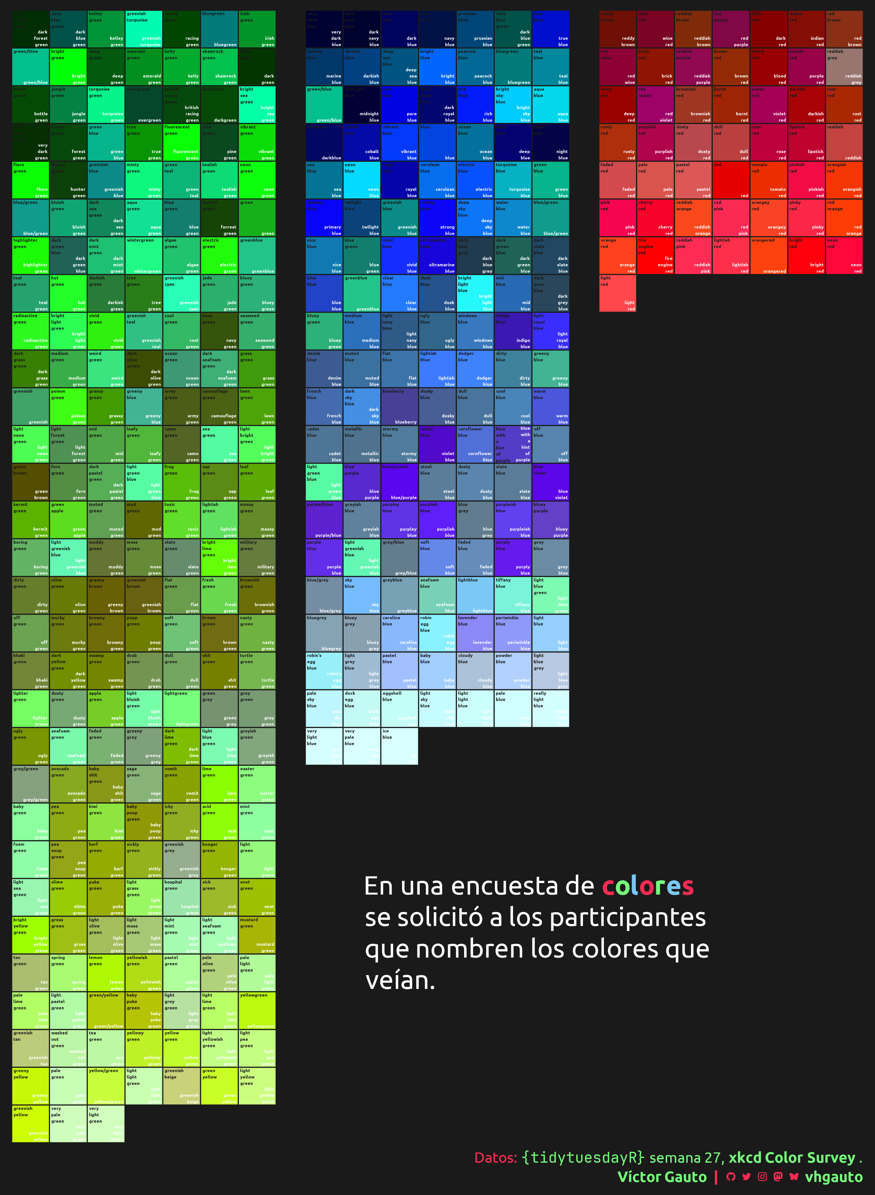
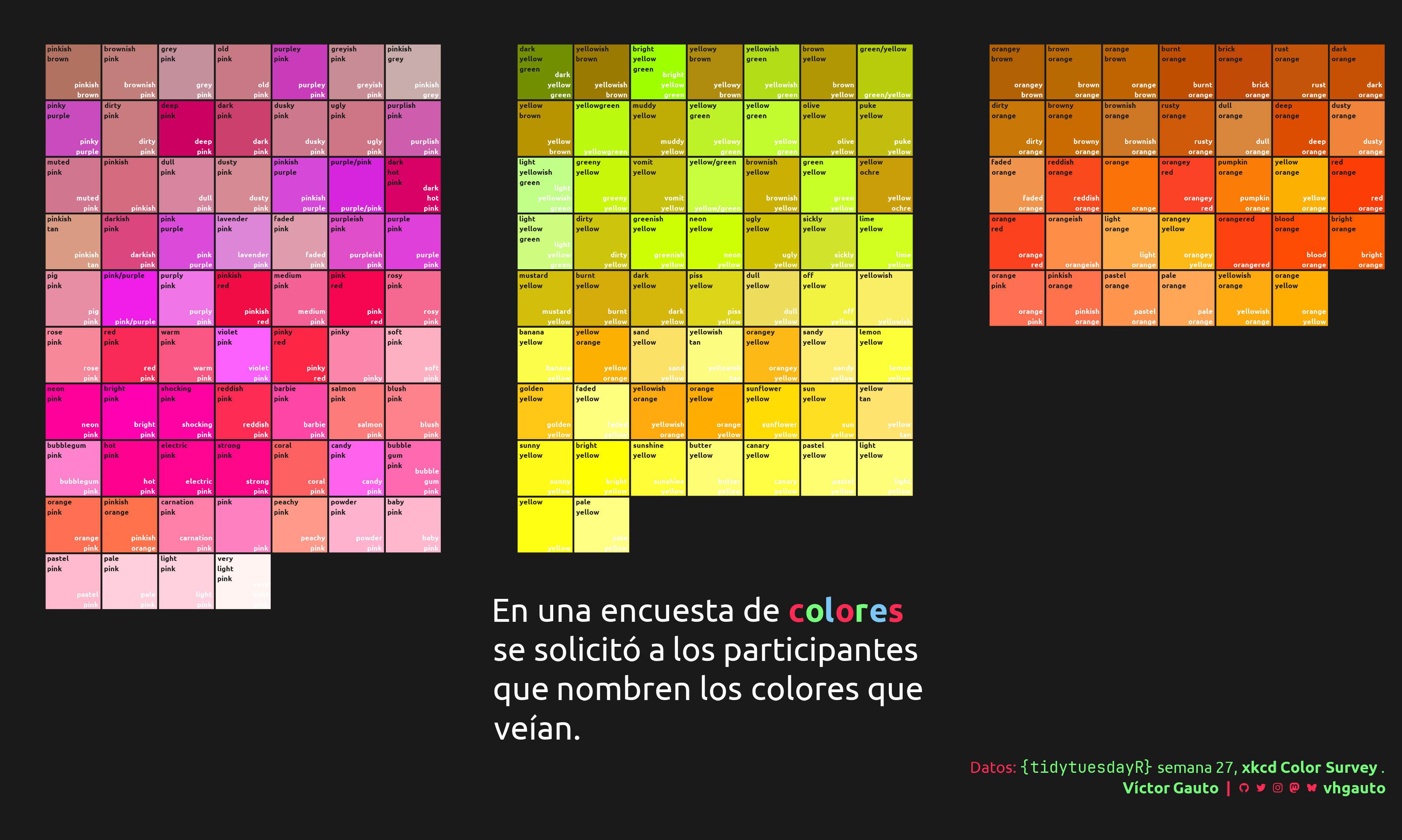
color_ranks <- tuesdata$color_ranksMe interesan los nombres que les dieron los encuestados a los colores, y poder visualizar los colores.
Defino dos funciones auxiliares. Función para asignar posiciones y el orden de los colores seleccionados.
f_color <- function(color_esp, color_eng, ancho = 7) {
  color_tbl <- color_ranks |>
    filter(str_detect(color, color_eng)) |>
    mutate(grupo = color_esp) |>
    mutate(rgb = map(hex, ~colorspace::hex2RGB(.x)@coords)) |>
    mutate(
      r = map_dbl(rgb, ~.x[1]),
      g = map_dbl(rgb, ~.x[2]),
      b = map_dbl(rgb, ~.x[3])
    ) |>
    arrange(r, g, b)

  n_ancho <- ancho
  n_alto <- ceiling(nrow(color_tbl)/n_ancho)

  expand_grid(
    y = 30:(30-n_alto),
    x = 1:n_ancho
  ) |>
    mutate(id = row_number()) |>
    filter(id <= nrow(color_tbl)) |>
    bind_cols(color_tbl)
}
Función para agregar un color diferente a cada letra.
f_label <- function(x) {
  n <- nchar(x)
  col <- rep(c(c3, c4, c5), length.out = n)
  l <- str_split(x, "")[[1]]
  glue(
    "<b style='color:{col}'>{l}</b>"
  ) |>
    str_flatten()
}
Identifico los colores de interés, genero la base de datos y reordeno los colores.
d <- bind_rows(
  f_color("azul", "blue"),
  f_color("rojo", "red"),
  f_color("verde", "green"),
) |>
  mutate(color = str_replace_all(color, " ", "\n")) |>
  mutate(grupo = factor(grupo, c("verde", "azul", "rojo")))
colores_label <- f_label("colores")Genero título y creo tibble para agregar a la figura de facetas.
mi_titulo <- glue(
  "En una encuesta de {colores_label}<br>se solicitó a los participantes<br>que
  nombren los colores que<br>veían."
)

mi_titulo_tbl <- tibble(
  x = 2,
  y = 6,
  label = mi_titulo,
  grupo = factor("azul")
)
Figura.
g <-  ggplot(d, aes(x, y, fill = hex)) +
  geom_tile(color = c1, linewidth = .5, show.legend = FALSE) +
  geom_text(
    aes(x = x-.45, y = y+.45, label = color), size = 1.5, hjust = 0, vjust = 1,
    family = "ubuntu", fontface = "bold", color = c1
  ) +
  geom_text(
    aes(x = x+.45, y = y-.45, label = color), size = 1.5, hjust = 1, vjust = 0,
    family = "ubuntu", fontface = "bold", color = c2
  ) +
  geom_richtext(
    data = mi_titulo_tbl, aes(x, y, label = label), family = "ubuntu", size = 9,
    color = c2, label.color = NA, inherit.aes = FALSE, hjust = 0,
    fill = NA
  ) +
  facet_wrap(vars(grupo), nrow = 1) +
  scale_fill_identity() +
  coord_equal(expand = FALSE, clip = "off") +
  labs(caption = mi_caption) +
  theme_void(base_family = "ubuntu", base_size = 18) +
  theme(
    plot.margin = margin(10, 10, 10, 10),
    plot.background = element_rect(fill = c1, color = NA),
    plot.title = element_markdown(),
    plot.caption = element_markdown(color = c3, lineheight = 1.3),
    panel.spacing.x = unit(1, "cm"),
    strip.text = element_blank()
  )
Guardo.
ggsave(
  plot = g,
  filename = "tidytuesday/2025/semana_27.png",
  width = 30,
  height = 41,
  units = "cm"
)