# paquetes ----------------------------------------------------------------
library(glue)
library(ggtext)
library(showtext)
library(patchwork)
library(tidyverse)
# fuente ------------------------------------------------------------------
# colores
c1 <- "grey80"
c2 <- "#8C0272"
c3 <- "#9B7424"
c4 <- "#A7F2F9"
# fuente: Ubuntu
font_add(
family = "ubuntu",
regular = "fuente/Ubuntu-Regular.ttf",
bold = "fuente/Ubuntu-Bold.ttf",
italic = "fuente/Ubuntu-Italic.ttf")
# fuente: Victor
font_add(
family = "victor",
regular = "fuente/VictorMono-ExtraLight.ttf",
bold = "fuente/VictorMono-VariableFont_wght.ttf",
italic = "fuente/VictorMono-ExtraLightItalic.ttf")
# íconos
font_add("fa-brands", "icon/Font Awesome 6 Brands-Regular-400.otf")
showtext_auto()
showtext_opts(dpi = 300)
# caption
fuente <- glue(
"Datos: <span style='color:{c3};'><span style='font-family:mono;'>",
"{{<b>tidytuesdayR</b>}}</span> semana {13}. ",
"NCAA Men's March Madness.</span>")
autor <- glue("<span style='color:{c3};'>**Víctor Gauto**</span>")
icon_twitter <- glue("<span style='font-family:fa-brands;'></span>")
icon_instagram <- glue("<span style='font-family:fa-brands;'></span>")
icon_github <- glue("<span style='font-family:fa-brands;'></span>")
icon_mastodon <- glue("<span style='font-family:fa-brands;'></span>")
usuario <- glue("<span style='color:{c3};'>**vhgauto**</span>")
sep <- glue("**|**")
mi_caption <- glue(
"{fuente}<br>{autor} {sep} {icon_github} {icon_twitter} {icon_instagram} ",
"{icon_mastodon} {usuario}")
# datos -------------------------------------------------------------------
tuesdata <- tidytuesdayR::tt_load(2024, 13)
team_results <- tuesdata$`team-results`
public_picks <- tuesdata$`public-picks`
# me interesan las expectativas del público y el historial de los equipos de
# la NCAA
# listado de equipos coincidentes en ambos datasets
equipos_interes <- inner_join(
select(team_results, TEAM),
select(public_picks, TEAM),
by = join_by(TEAM)
) |>
pull()
# etiquetas de las rondas
eje_x_label <- c(
"32<sup>avos</sup><br>|<br>|<br>|<br>|<br>|<br>|",
"16<sup>avos</sup><br>|<br>|<br>|<br>|<br>|",
"8<sup>avos</sup><br>|<br>|<br>|<br>|",
"4<sup>tos</sup><br>|<br>|<br>|",
"Semi<br>|<br>|",
"<span style='font-size:17px;'>Final</span>")
# expectativas, en porcentajes
d_expectativa <- public_picks |>
filter(TEAM %in% equipos_interes) |>
select(TEAM, R64, R32, S16, E8, F4, FINALS) |>
mutate(
across(
.cols = -TEAM,
.fns = ~ str_remove(.x, "%") |> as.numeric()
)
) |>
pivot_longer(
cols = -TEAM,
names_to = "pos",
values_to = "valor"
) |>
mutate(pos = fct(
pos,
levels = c("R64", "R32", "S16", "E8", "F4", "FINALS"))) |>
rename(equipo = TEAM) |>
mutate(s = sum(valor), .by = equipo) |>
mutate(equipo = fct_reorder(equipo, s)) |>
mutate(eje_x = as.numeric(pos)) |>
mutate(tipo = "expectativa") |>
select(equipo, valor, eje_x, tipo) |>
filter(as.numeric(equipo) >= 29)
# historial, en cantidad de partidos
d_historia <- team_results |>
filter(TEAM %in% equipos_interes) |>
select(TEAM, R64, R32, S16, E8, F4, CHAMP) |>
pivot_longer(
cols = -TEAM,
names_to = "pos",
values_to = "valor"
) |>
mutate(suma = sum(valor), .by = TEAM) |>
mutate(TEAM = fct_reorder(TEAM, suma)) |>
select(equipo = TEAM, pos, valor) |>
mutate(pos = fct(
pos,
levels = c("R64", "R32", "S16", "E8", "F4", "CHAMP"))) |>
mutate(s = sum(valor), .by = equipo) |>
mutate(eje_x = as.numeric(pos)) |>
mutate(tipo = "historia") |>
select(equipo, valor, eje_x, tipo) |>
filter(as.numeric(equipo) >= 29)
# figura ------------------------------------------------------------------
# heatmap de las expectativas
g_expectativa <- ggplot(d_expectativa, aes(eje_x, equipo, fill = valor)) +
geom_tile(color = c1, linewidth = 1) +
scale_x_continuous(
breaks = 1:6, sec.axis = dup_axis(
labels = eje_x_label
)) +
scico::scale_fill_scico(
palette = "hawaii",
breaks = seq(0, 100, 25),
limits = c(0, 100),
labels = (x) glue("{x}%")) +
coord_equal() +
labs(
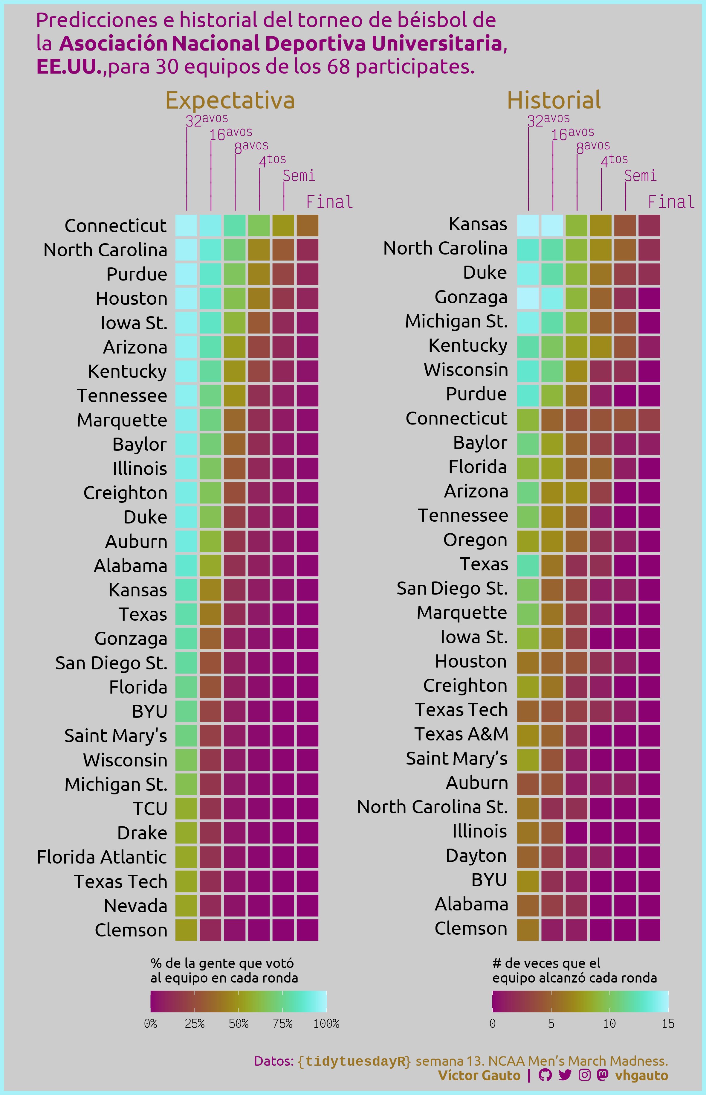
x = NULL, y = NULL, title = "Expectativa",
fill = "% de la gente que votónal equipo en cada ronda") +
guides(fill = guide_colorbar(title.position = "top")) +
theme_void() +
theme(
plot.title = element_text(
family = "ubuntu", color = c3, size = 20, hjust = 0),
axis.text.x.top = element_markdown(
vjust = 0, hjust = 0, color = c2, family = "victor"),
axis.text.y = element_text(family = "ubuntu", hjust = 1, size = 15),
legend.position = c(1, 0),
legend.justification = c(1, 1),
legend.direction = "horizontal",
legend.title = element_text(family = "ubuntu", margin = margin(t = 10)),
legend.key.width = unit(10, "mm"),
legend.text = element_text(family = "victor")
)
# heatmap del historial
g_historia <- ggplot(d_historia, aes(eje_x, equipo, fill = valor)) +
geom_tile(color = c1, linewidth = 1) +
scale_x_continuous(
breaks = 1:6, sec.axis = dup_axis(
labels = eje_x_label
)) +
scico::scale_fill_scico(
palette = "hawaii",
breaks = seq(0, 15, 5)) +
coord_equal() +
labs(
x = NULL, y = NULL, title = "Historial",
fill = "# de veces que elnequipo alcanzó cada ronda") +
guides(fill = guide_colorbar(title.position = "top")) +
theme_void() +
theme(
plot.title = element_text(
family = "ubuntu", color = c3, size = 20, hjust = 0),
axis.text.x.top = element_markdown(
vjust = 0, hjust = 0, color = c2, family = "victor"),
axis.text.y = element_markdown(
family = "ubuntu", hjust = 1, margin = margin(l = 25), size = 15),
legend.position = c(1, 0),
legend.justification = c(1, 1),
legend.direction = "horizontal",
legend.title = element_text(family = "ubuntu", margin = margin(t = 10)),
legend.key.width = unit(10, "mm"),
legend.text = element_text(family = "victor")
)
# combino ambas figuras
g <- g_expectativa + g_historia +
plot_annotation(
subtitle = glue(
"Predicciones e historial del torneo de béisbol de<br>",
"la **Asociación Nacional Deportiva Universitaria**,<br>",
"**EE.UU.**,para 30 equipos de los 68 participates.",
),
caption = mi_caption,
theme = theme(
plot.margin = margin(t = 10, r = 30, l = 30),
plot.background = element_rect(
fill = c1, color = c4, linewidth = 3),
plot.title.position = "plot",
plot.subtitle = element_markdown(
family = "ubuntu", size = 17, color = c2, hjust = 0,
lineheight = unit(1.1, "line")),
plot.caption = element_markdown(
color = c2, family = "ubuntu", size = 11,
margin = margin(t = 90, b = 10))
)
)
# guardo
ggsave(
plot = g,
filename = "2024/s13/viz.png",
width = 20,
height = 31,
units = "cm")
# abro
browseURL("2024/s13/viz.png")