Semana 41

Figura semana 41

Especies nativas y no nativas en Parques Nacionales de EE.UU.

Script

# paquetes ----------------------------------------------------------------

library(glue)
library(ggtext)
library(showtext)
library(tidytext)
library(tidyverse)

# fuente ------------------------------------------------------------------

# colores
c1 <- "#6B200C"
c2 <- "#5A5A83"
c3 <- "#000000"
c4 <- "#FBE3C2"
c5 <- "grey20"

# fuente: Ubuntu
font_add(
  family = "ubuntu", 
  regular = "fuente/Ubuntu-Regular.ttf",
  bold = "fuente/Ubuntu-Bold.ttf",
  italic = "fuente/Ubuntu-Italic.ttf"
)

# monoespacio & íconos
font_add(
  family = "jet", 
  regular = "fuente/JetBrainsMonoNLNerdFontMono-Regular.ttf"
)

# bebas neuw
font_add_google(
  name = "Bebas Neue",
  family = "bebas neue"
)

showtext_auto()
showtext_opts(dpi = 300)

# caption
fuente <- glue(
  "Datos: <span style='color:{c2};'><span style='font-family:jet;'>",
  "{{<b>tidytuesdayR</b>}}</span> semana {41}, ",
  "<b>NPSpecies - The National Park Service biodiversity database</b>.</span>"
)
autor <- glue("<span style='color:{c2};'>**Víctor Gauto**</span>")
icon_twitter <- glue("<span style='font-family:jet;'>&#xf099;</span>")
icon_instagram <- glue("<span style='font-family:jet;'>&#xf16d;</span>")
icon_github <- glue("<span style='font-family:jet;'>&#xf09b;</span>")
icon_mastodon <- glue("<span style='font-family:jet;'>&#xf0ad1;</span>")
usuario <- glue("<span style='color:{c2};'>**vhgauto**</span>")
sep <- glue("**|**")

mi_caption <- glue(
  "{fuente}<br>{autor} {sep} {icon_github} {icon_twitter} {icon_instagram} ",
  "{icon_mastodon} {usuario}"
)

# datos -------------------------------------------------------------------

tuesdata <- tidytuesdayR::tt_load(2024, 41)
nps <- tuesdata$most_visited_nps_species_data

# me interesa la cantidad de algunas especies por cada parque, y si son
# nativas o no

# especies de interés y su traducción
animales <- c(
  "Amphibian", "Bird", "Fish", "Fungi", "Insect", "Mammal", "Reptile"
)
animales_trad <- c(
  "Anfibio", "Ave", "Pez", "Fungi", "Insecto", "Mamífero", "Reptil"
)
names(animales_trad) <- animales

# filtro por las especies de interés y agrego traducciones
d <- nps |> 
  select(ParkName, CategoryName, Nativeness) |> 
  drop_na() |> 
  filter(Nativeness != "Unknown") |> 
  count(ParkName, CategoryName, Nativeness) |> 
  arrange(ParkName, desc(n)) |> 
  mutate(ParkName = str_remove(ParkName, " National Park")) |> 
  filter(n > 1) |> 
  filter(CategoryName %in% animales) |> 
  mutate(CategoryName = animales_trad[CategoryName]) |> 
  mutate(ParkName = glue("{icon_parque} {ParkName} {icon_parque}"))

# figura ------------------------------------------------------------------

# ícono para el nombre del parque
icon_parque <- glue(
  "<span style='font-family:jet; font-size: 30px; color: {c1}'>&#xf185;</span>"
)

# subtítulo
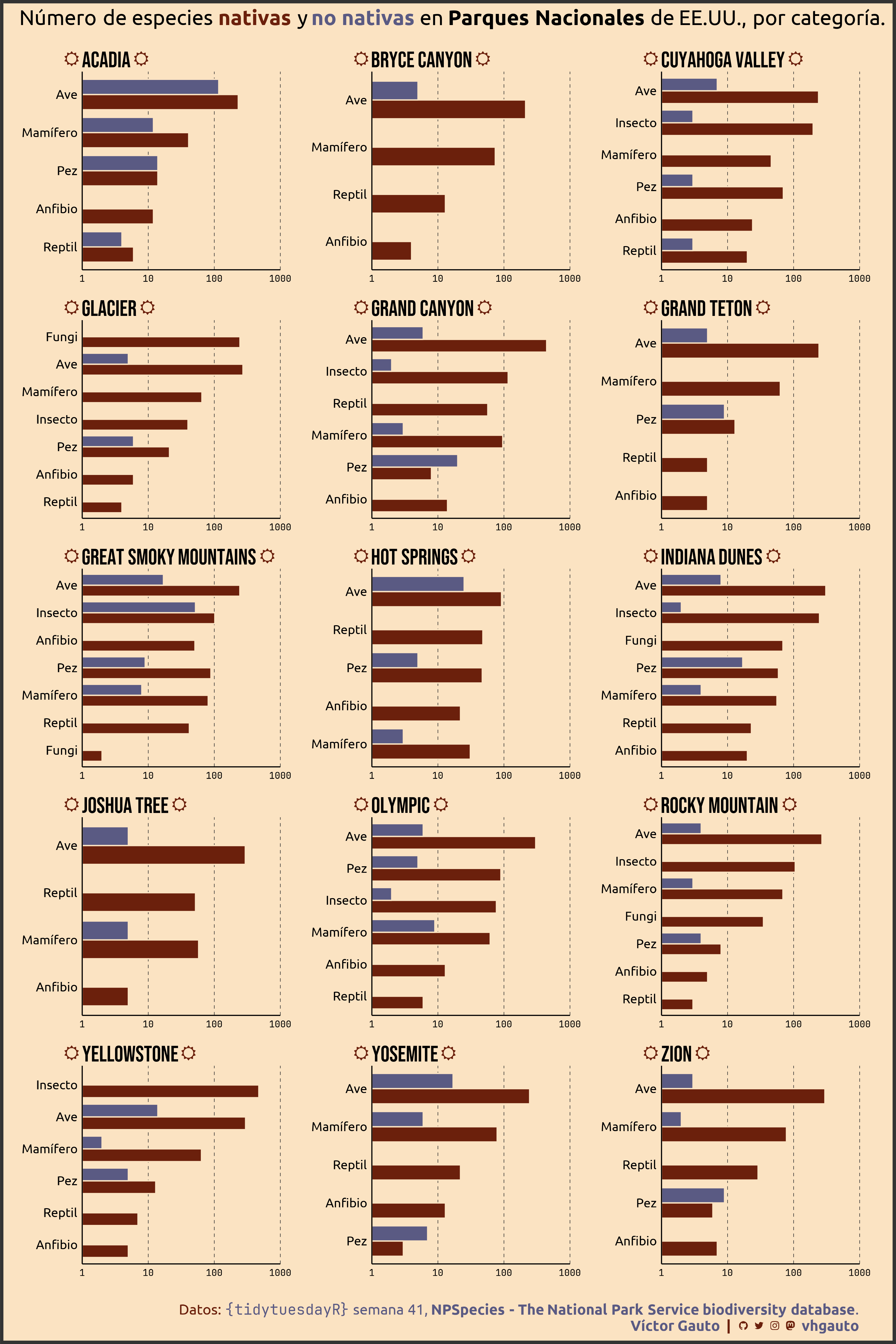
mi_subtitulo <- glue(
  "Número de especies <b style='color: {c1}'>nativas</b> y ",
  "<b style='color: {c2}'>no nativas</b> en <b>Parques Nacionales</b> ",
  "de EE.UU., por categoría."
)

# figura
# uso 'reorder_within()' junto con 'scale_y_reordered()' para ordenar
# categorías que se repiten en los paneles
g <- ggplot(
  d, 
  aes(n, reorder_within(CategoryName, n, ParkName), fill = Nativeness)) +
  geom_col(
    position = position_dodge(preserve = "single"), width = .8,
    show.legend = FALSE, color = c4, linewidth = .6
  ) +
  facet_wrap(vars(ParkName), scales = "free", ncol = 3) +
  scale_y_reordered() +
  scale_x_log10(limits = c(1, 1000), expand = c(0, 0)) +
  scale_fill_manual(
    breaks = c("Native", "Non-native"),
    values = c(c1, c2)
  ) +
  coord_cartesian(clip = "off") +
  labs(
    x = NULL, y = NULL, fill = NULL, caption = mi_caption,
    subtitle = mi_subtitulo
  ) +
  theme_classic() +
  theme(
    aspect.ratio = 1,
    plot.margin = margin(l = 20, r = 34.6),
    plot.background = element_rect(fill = c4, color = c5, linewidth = 3),
    plot.title.position = "plot",
    plot.subtitle = element_markdown(
      family = "ubuntu", size = 20, margin = margin(t = 10, b = 20)
    ),
    plot.caption = element_markdown(
      color = c1, family = "ubuntu", size = 14,
      margin = margin(t = 25, b = 10), lineheight = unit(1.1, "line")
    ),
    panel.background = element_blank(),
    panel.grid.minor = element_blank(),
    panel.grid.major.y = element_blank(),
    panel.grid.major.x = element_line(
      linetype = "66", linewidth = .25, color = c5
    ),
    panel.spacing.x = unit(2, "line"),
    panel.spacing.y = unit(1, "line"),
    axis.text.x = element_text(family = "jet", color = c3),
    axis.text.y = element_text(family = "ubuntu", color = c3, size = 12),
    axis.ticks = element_blank(),
    strip.background = element_blank(),
    strip.text = element_markdown(
      family = "bebas neue", size = 21, hjust = 0, margin = margin(l = -17),
      color = c3
    )
  )

# guardo
ggsave(
  plot = g,
  filename = "2024/s41/viz.png",
  width = 30,
  height = 45,
  units = "cm")

# abro
browseURL(glue("{getwd()}/2024/s41/viz.png"))

Figura