Semana 22

Figura semana 22

Plantaciones por lote y año del paquete {gardenR}

Script

# paquetes ----------------------------------------------------------------

library(glue)
library(ggtext)
library(showtext)
library(sf)
library(tidyverse)

# fuente ------------------------------------------------------------------

# colores
c1 <- "#A71B4B"
c2 <- "#22C4B3"
c3 <- "#584B9F"
c4 <- "grey95"
c5 <- "grey20"
c6 <- "white"

# fuente: Ubuntu
font_add(
  family = "ubuntu", 
  regular = "fuente/Ubuntu-Regular.ttf",
  bold = "fuente/Ubuntu-Bold.ttf",
  italic = "fuente/Ubuntu-Italic.ttf")

# monoespacio & íconos
font_add(
  family = "jet", 
  regular = "fuente/JetBrainsMonoNLNerdFontMono-Regular.ttf")

# bebas neue
font_add(
  family = "bebas",
  regular = "fuente/BebasNeue-Regular.ttf"
)

showtext_auto()
showtext_opts(dpi = 300)

# caption
fuente <- glue(
  "Datos: <span style='color:{c3};'><span style='font-family:jet;'>",
  "{{<b>tidytuesdayR</b>}}</span> semana {22}, ",
  "<b>Lisa Lendway</b>, <span style='font-family:jet;'>{{gardenR}}</span>.",
  "</span>")
autor <- glue("<span style='color:{c3};'>**Víctor Gauto**</span>")
icon_twitter <- glue("<span style='font-family:jet;'>&#xf099;</span>")
icon_instagram <- glue("<span style='font-family:jet;'>&#xf16d;</span>")
icon_github <- glue("<span style='font-family:jet;'>&#xf09b;</span>")
icon_mastodon <- glue("<span style='font-family:jet;'>&#xf0ad1;</span>")
usuario <- glue("<span style='color:{c3};'>**vhgauto**</span>")
sep <- glue("**|**")

mi_caption <- glue(
  "{fuente}<br>{autor} {sep} {icon_github} {icon_twitter} {icon_instagram} ",
  "{icon_mastodon} {usuario}")

# datos -------------------------------------------------------------------

tuesdata <- tidytuesdayR::tt_load(2024, 22)
garden_coords <- gardenR::garden_coords

# me interesan las plantaciones por año, sobre los lotes

# combino los datos de 2020 y 2021
planting_2020 <- tuesdata$planting_2020
planting_2021 <- tuesdata$planting_2021

planting <- bind_rows(
  planting_2020 |> mutate(año = 2020),
  planting_2021 |> mutate(año = 2021)
) |> 
  mutate(vegetable = case_match(
    vegetable,
    "pumpkins" ~ "pumpkin",
    .default = vegetable
  )) |> 
  mutate(plot = str_remove(plot, "pot")) |> 
  filter(plot %in% unique(garden_coords$plot))

# función que genera un sf a partir de las coordenadas de los lotes
f_plot <- function(plot_id) {
  p <- filter(garden_coords, plot == plot_id)
  
  v <- st_cast(st_linestring(cbind(p$x, p$y)),"POLYGON") |> 
    st_sfc() |> 
    st_sf() |> 
    rename("geom" = 1) |> 
    mutate(plot = plot_id, .before = 1)
  
  return(v)
}

# a partir de la cantidad de plantaciones agrego puntos sobre los lotes
f_puntos <- function(x_año, y_plot) {
  y <- filter(planting, año == x_año) |> 
    reframe(
      s = sum(number_seeds_planted, na.rm = TRUE),
      .by = plot
    ) |> 
    inner_join(
      plot_sf,
      by = join_by(plot)
    ) |> 
    filter(plot == y_plot) |> 
    st_sf()
  
  p <- st_sample(y, size = y$s) |> 
    st_sf() |> 
    rename(geom = 1) |> 
    mutate(plot = y_plot, .before = 1) |> 
    mutate(año = x_año)
  
  return(p)
  
}

# sf delos lotes
plot_sf <- map(unique(garden_coords$plot), f_plot) |> 
  list_rbind() |> 
  st_sf()

# combino las plantaciones de 2020 y 2021
plot_2020 <- filter(planting, año == 2020) |> 
  drop_na(number_seeds_planted) |> 
  distinct(plot) |> 
  pull()

plot_2021 <- filter(planting, año == 2021) |> 
  drop_na(number_seeds_planted) |> 
  distinct(plot) |> 
  pull()

p_2020 <- map2(
  .x = rep(2020, length(plot_2020)),
  .y = plot_2020,
  ~ f_puntos(x_año = .x, y_plot = .y)
) |> 
  list_rbind() |> 
  st_sf()

p_2021 <- map2(
  .x = rep(2021, length(plot_2021)),
  .y = plot_2021,
  ~ f_puntos(x_año = .x, y_plot = .y)
) |> 
  list_rbind() |> 
  st_sf()

p <- rbind(p_2020, p_2021)

# extensión de los lotes
plot_bb <- st_as_sfc(st_bbox(plot_sf))

# cantidad de semillas plantadas por año
n_año <- planting |> 
  reframe(
    s = sum(number_seeds_planted, na.rm = TRUE),
    .by = año
  ) |> 
  mutate(
    label = glue("\# de semillas plantadas = <b style='color:{c1}'>{s}</b>")
  )

# figura ------------------------------------------------------------------

# paleta de colores
pal <- hcl.colors(
  n = length(unique(garden_coords$plot)), 
  palette = "Zissou 1") |> 
  sample()

# título y subtítulo
mi_subtitle <- glue(
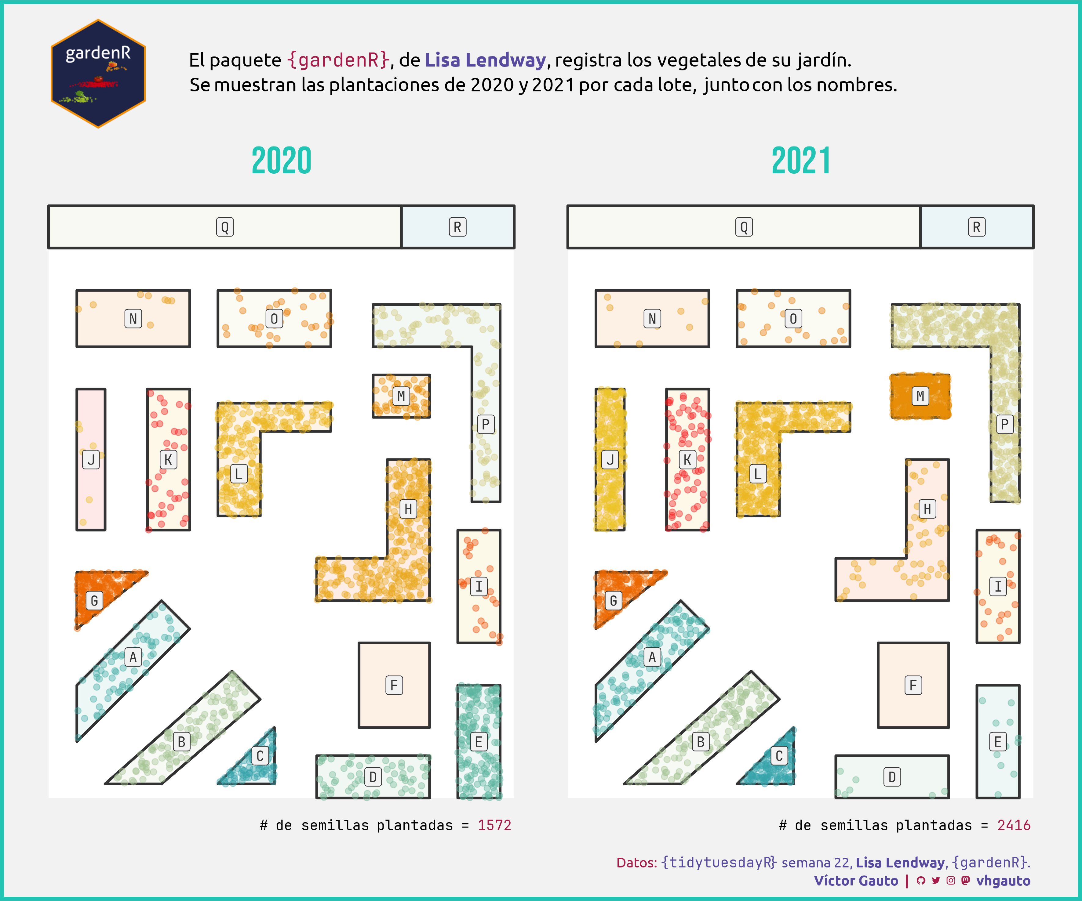
  "El paquete <span style='font-family:jet; color:{c1}'>{{gardenR}}</span>, ",
  "de <b style='color:{c3}'>Lisa Lendway</b>, registra los vegetales de su ",
  "jardín.<br>",
  "Se muestran las plantaciones de 2020 y 2021 por cada lote, junto con los ",
  "nombres."
)

# logo de {gardenR}
logo_url <- "https://raw.githubusercontent.com/llendway/gardenR/main/man/figures/logo.png"
mi_title <- glue("<img src={logo_url} width=75 />")

# figura
g <- ggplot() +
  # extensión
  geom_sf(
    data = plot_bb, fill = c6, color = NA
  ) +
  # lotes
  geom_sf(
    data = plot_sf, aes(fill = plot, color = plot), alpha = .1, linewidth = 1,
    color = c5
  ) +
  # plantaciones
  geom_sf(
    data = p, aes(color = plot), alpha = .4, size = 2
  ) +
  # nombre de los lotes
  geom_sf_label(
    data = plot_sf, aes(label = plot), family = "jet", fill = c4, color = c5
  ) +
  geom_richtext(
    data = n_año, aes(x = 17.5, y = 1, label = label), family = "jet", 
    hjust = .1, fill = NA, label.color = NA
  ) +
  facet_wrap(vars(año), nrow = 1) +
  scale_fill_manual(values = pal) +
  scale_color_manual(values = pal) +
  labs(subtitle = mi_subtitle, caption = mi_caption, title = mi_title) +
  theme_void() +
  theme(
    plot.margin = margin(t = 4.6, r = 20, b = 0, l = 20),
    plot.background = element_rect(fill = c4, color = c2, linewidth = 3),
    plot.title = element_markdown(margin = margin(b = -70, l = 20, t = 10)),
    plot.subtitle = element_markdown(
      family = "ubuntu", size = 15, lineheight = unit(1.3, "line"),
      margin = margin(b = 40, t = 10, l = 130)),
    plot.caption = element_markdown(
      family = "ubuntu", color = c1, size = 11, lineheight = unit(1.3, "line"),
      margin = margin(b = 10, r = 20)),
    strip.text = element_text(family = "bebas", size = 30, color = c2),
    legend.position = "none"
  )

# guardo
ggsave(
  plot = g,
  filename = "2024/s22/viz.png",
  width = 30,
  height = 25,
  units = "cm")

# abro
browseURL("2024/s22/viz.png")

Figura