Semana 16

Figura semana 16

Alimentación del período Neolítico.

Script

# paquetes ----------------------------------------------------------------

library(tidyverse)
library(sf)
library(ggrepel)
library(glue)
library(ggtext)
library(showtext)
library(fontawesome)

# fuentes -----------------------------------------------------------------

font_add_google(name = "Poltawski Nowy", family = "poltawski", db_cache = FALSE) # título
font_add_google(name = "Anuphan", family = "anuphan", db_cache = FALSE) # resto del texto
font_add_google(name = "Share Tech Mono", family = "share", db_cache = FALSE) # coordenadas

showtext_auto()
showtext_opts(dpi = 300)

# íconos
font_add("fa-reg", "icon/Font Awesome 5 Free-Regular-400.otf")
font_add("fa-brands", "icon/Font Awesome 5 Brands-Regular-400.otf")
font_add("fa-solid", "icon/Font Awesome 5 Free-Solid-900.otf")

# caption
icon_twitter <- "<span style='font-family:fa-brands;'>&#xf099;</span>"
icon_github <- "<span style='font-family:fa-brands;'>&#xf09b;</span>"
fuente <- "Datos: <span style='color:#a41400;'><span style='font-family:mono;'>{**tidytuesdayR**}</span> semana 16</span>"
autor <- "Autor: <span style='color:#a41400;'>**Víctor Gauto**</span>"
sep <- glue("**|**")
usuario <- glue("<span style='color:#a41400;'>**vhgauto**</span>")

mi_caption <- glue("{fuente} {sep} {autor} {sep} {icon_github} {icon_twitter} {usuario}")

# datos -------------------------------------------------------------------

browseURL("https://github.com/rfordatascience/tidytuesday/blob/master/data/2023/2023-04-18/readme.md")

founder_crops <- readr::read_csv('https://raw.githubusercontent.com/rfordatascience/tidytuesday/master/data/2023/2023-04-18/founder_crops.csv')

# convierto las coordenadas a sf
founder_crops_sf <- st_as_sf(founder_crops,
                             coords = c("longitude", "latitude"),
                             crs = st_crs(4326))

# mapa del mundo
world <- rnaturalearth::ne_countries(scale = "medium", returnclass = "sf")

# región de interés, bbox de la base de datos
l <- st_bbox(founder_crops_sf) |> 
  st_as_sfc() |> 
  st_as_sf()

# evito errores al recortar el mapa del mundo
sf_use_s2(FALSE)

# recorto el mapa del mundo a la base de datos
world_subset <- st_crop(world, l)

# me interesan las ubicaciones y 'comestibilidad', solo tomo datos únicos
# incluye 'Edible seed/fruit'
sub <- founder_crops_sf |> 
  drop_na(edibility) |> 
  distinct(geometry, edibility) |>  
  mutate(edibility2 = fct_lump_n(f = edibility, n = 3))

# remuevo la categoría que se repite en TODOS los puntos (Edible seed/fruit)
# conservo las restantes, elijo las 3 más frecuentes y lump el resto
sub2 <- founder_crops_sf |> 
  # remuevo NA
  drop_na(edibility) |> 
  # mantengo ubicaciones únicas
  distinct(geometry, edibility) |> 
  # remuevo la categoría que se repite en todas las ubicaciones
  filter(edibility != "Edible seed/fruit") |> 
  # lump categorías poco frecuentes
  mutate(edibility2 = fct_lump_n(
    f = edibility, 
    n = 3, 
    ties.method = "first",
    other_level = "Otros")) |>
  # traduzco
  mutate(edibility2 = case_match(
    edibility2,
    "leaves, stems" ~ "Hoja, tallo",
    "flowers, stems" ~ "Flor, tallo",
    "leaves, root" ~ "Hoja, raíz", 
    .default = edibility2))

# categoría Otros
sub3 <- sub2 |> 
  filter(edibility2 == "Otros") |> 
  mutate(edibility = case_match(
    edibility,
    "stems" ~ "Tallo",
    "rhizomes, stems and leaves," ~ "Rizoma, tallo, hoja",
    "bulbs" ~ "Bulbo",
    "flowers" ~ "Flor",
    "leaves" ~ "Hoja",
    .default = edibility))

# figura ------------------------------------------------------------------

# función p/colorear palabras
f_c <- function(x) {
  glue("<span style='color:#a41400'>**{x}**</span>")
}

# figura
g1 <- sub2 |> 
  ggplot() +
  # mundo
  geom_sf(data = world_subset, fill = "grey90", color = "grey20", 
          linewidth = .2, linetype = 2) +
  # todos los puntos
  geom_sf(data = sub |> select(-edibility2),
          color = "#007e2e", alpha = 1, size = 1) +
  # puntos de las facetas
  geom_sf(alpha = .8, color = "#a41400", size = 3, show.legend = TRUE) +
  # otros
  geom_label_repel(
    data = sub3,
    aes(label = edibility, geometry = geometry),
    color = "#59386c",
    label.size = 0,
    label.padding = unit(.1, "line"),
    fill = alpha("white", .75),
    stat = "sf_coordinates",
    force = 7,
    size = 4.25,
    family = "anuphan",
    max.overlaps = 20,
    min.segment.length = 0) +
  # manual
  coord_sf(expand = FALSE, clip = "off") +
  labs(x = NULL, y = NULL, 
       title = "Dieta neolítica",
       subtitle = glue(
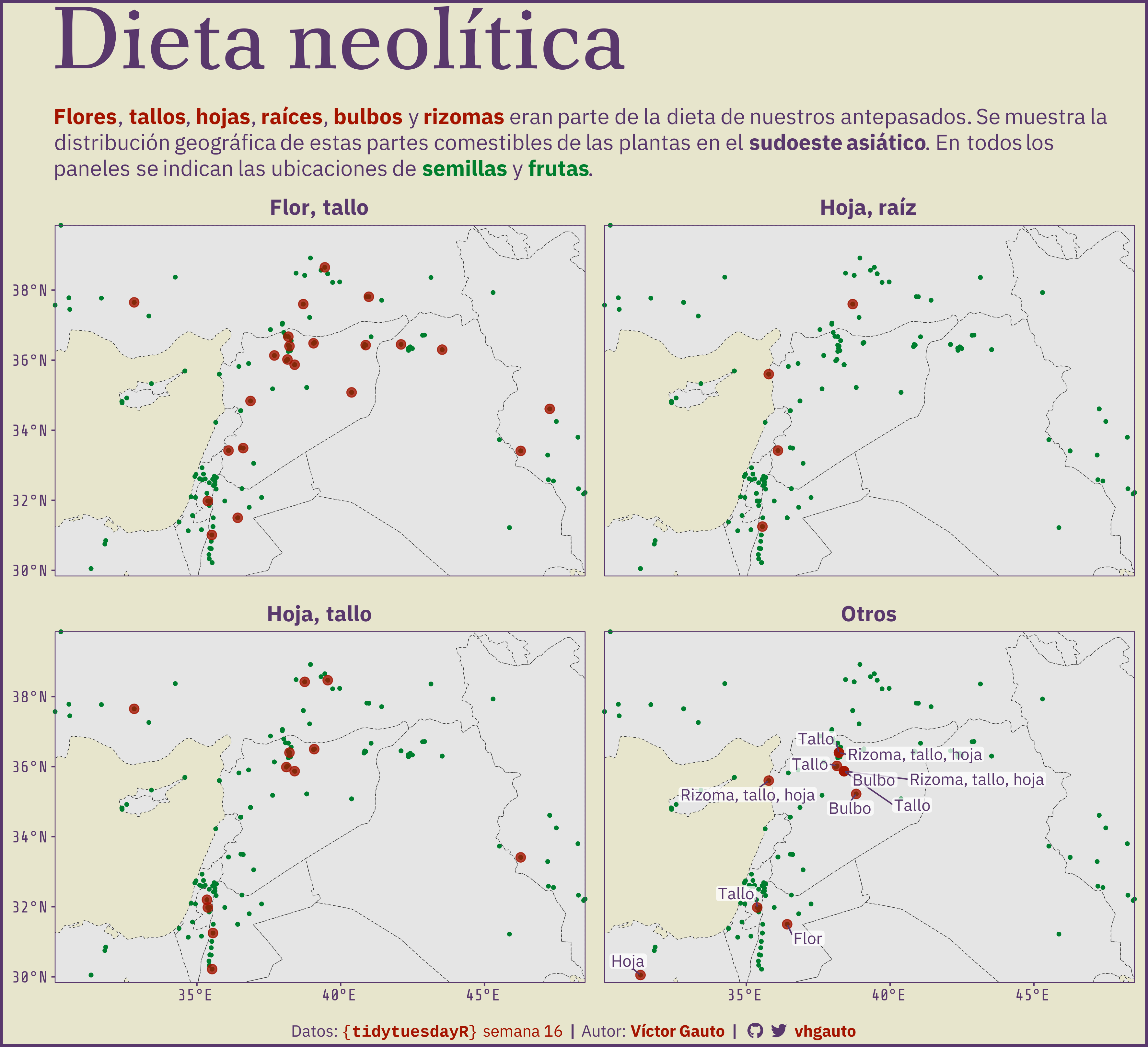
         " {f_c('Flores')}, {f_c('tallos')}, {f_c('hojas')}, {f_c('raíces')}, 
         {f_c('bulbos')} y {f_c('rizomas')} eran parte de la dieta de nuestros 
         antepasados. Se muestra la distribución geográfica de estas partes 
         comestibles de las plantas en el **sudoeste asiático**. En todos los 
         paneles se indican las ubicaciones de 
         <span style='color:#007e2e'>**semillas**</span> y 
         <span style='color:#007e2e'>**frutas**</span>."),
       caption = mi_caption) +
  # faceta
  facet_wrap(~ edibility2, ncol = 2, nrow = 2) +
  # tema
  theme_minimal() +
  theme(
    plot.background = element_rect(
      fill = "#e7e5cc", color = "#59386c", linewidth = 2),
    plot.title.position = "panel",
    plot.title = element_markdown(
      size = 65, family = "poltawski", color = "#59386c"),
    plot.subtitle = element_textbox_simple(
      size = 16, family = "anuphan", color = "#59386c", 
      margin = margin(10, 0, 10, 0)),
    plot.caption = element_markdown(
      size = 12, hjust = .46, family = "anuphan", margin = margin(15, 0, 5, 0),
      color = "#59386c"),
    plot.margin = margin(5, 10, 0, 10),
    strip.text = element_markdown(
      family = "anuphan", size = 16, color = "#59386c", face = "bold"),
    axis.text = element_markdown(family = "share", size = 12, color = "#59386c"),
    axis.ticks = element_line(color = "#59386c"),
    panel.grid = element_blank(),
    panel.ontop = TRUE,
    panel.background = element_rect(fill = NA, color = "#59386c", linewidth = .3),
    panel.spacing.x = unit(1, "line"),
    panel.spacing.y = unit(1.25, "line"))

# guardo
ggsave(
  plot = g1,
  filename = "2023/semana_16/viz.png",
  width = 30,
  height = 27.37,
  units = "cm",
  dpi = 300)

# abro
browseURL("2023/semana_16/viz.png")

Figura