Ocultar código
library(glue)
library(ggtext)
library(showtext)
library(tidyverse)Falta de acceso al agua en EE.UU.
library(glue)
library(ggtext)
library(showtext)
library(tidyverse)Colores
c1 <- "#4060C8"
c2 <- "#9A153D"
c3 <- "#EAF3FF"
c4 <- "grey50"
Fuentes: Ubuntu y JetBrains Mono
font_add(
  family = "ubuntu",
  regular = "././fuente/Ubuntu-Regular.ttf",
  bold = "././fuente/Ubuntu-Bold.ttf",
  italic = "././fuente/Ubuntu-Italic.ttf"
)

font_add(
  family = "jet",
  regular = "././fuente/JetBrainsMonoNLNerdFontMono-Regular.ttf"
)

showtext_auto()
showtext_opts(dpi = 300)fuente <- glue(
"Datos: <span style='color:{c1};'><span style='font-family:jet;'>",
"{{<b>tidytuesdayR</b>}}</span> semana 04, ",
"<b>U.S. Census Bureau</b>, {{tidycensus}}.</span>"
)
autor <- glue("<span style='color:{c1};'>**Víctor Gauto**</span>")
icon_twitter <- glue("<span style='font-family:jet;'></span>")
icon_instagram <- glue("<span style='font-family:jet;'></span>")
icon_github <- glue("<span style='font-family:jet;'></span>")
icon_mastodon <- glue("<span style='font-family:jet;'>󰫑</span>")
icon_bsky <- glue("<span style='font-family:jet;'></span>")
usuario <- glue("<span style='color:{c1};'>**vhgauto**</span>")
sep <- glue("**|**")
mi_caption <- glue(
"{fuente}<br>{autor} {sep} {icon_github} {icon_twitter} {icon_instagram} ",
"{icon_mastodon} {icon_bsky} {usuario}"
)tuesdata <- tidytuesdayR::tt_load(2025, 04)
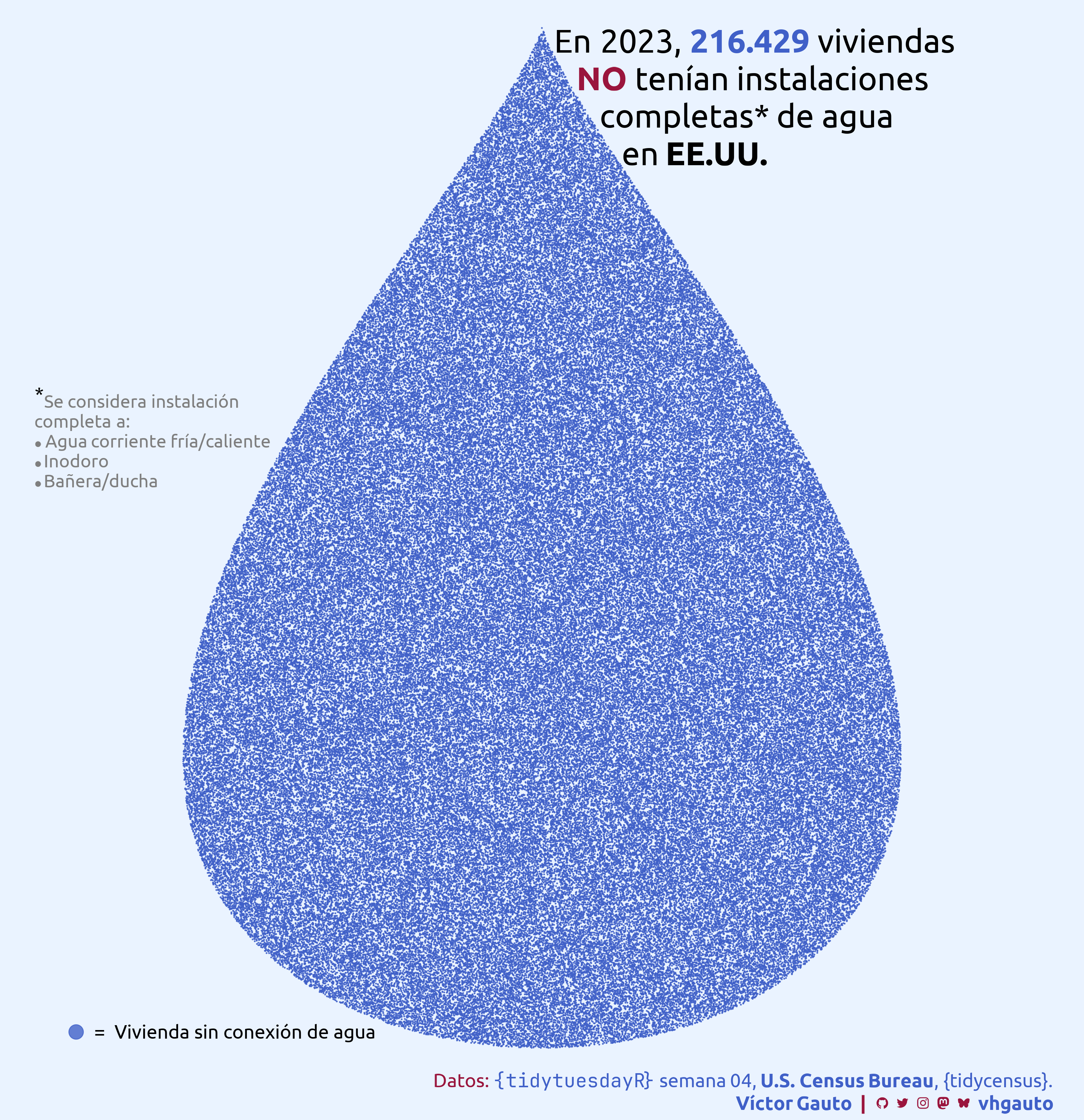
w23 <- tuesdata$water_insecurity_2023Me interesa ver la cantidad de gente SIN conexión a agua potable en 2023.
Cantidad total de viviendas SIN conexión, y formato para subtítulo
s23 <- sum(w23$plumbing, na.rm = TRUE)
s23_formato <- format(s23, big.mark = ".", decimal.mark = ",")
Tibble que generan puntos con forma de gota y convierto a vector.
Ecuación: Teardrop Curve.
gota_tbl <- tibble(
  t = seq(-10, 10, length.out = 1000),
  x_eje = cos(t),
  y_eje = sin(t)*sin(t/2)^1.5
) |>
  transmute(
    y = x_eje,
    x = -y_eje
  ) |>
  drop_na()

gota_v <- terra::vect(gota_tbl, geom = c("x", "y")) |>
  terra::as.lines() |>
  terra::aggregate() |>
  terra::as.polygons()
Dentro de la gota agrego puntos aleatoriamente, extraigo las coordenadas para usar con ggplot(). La cantidad de puntos es la de viviendas SIN conexión
p23 <- terra::spatSample(gota_v, s23) |>
terra::geom(df = TRUE)Subtítulo, rodeando la gota
l1 <- glue("En 2023, <b style='color:{c1}'>{s23_formato}</b> viviendas")
l2 <- glue("<b style='color:{c2}'>NO</b> tenían instalaciones")
l3 <- "completas* de agua"
l4 <- "en <b>EE.UU.</b>"
mi_subtitulo <- c(l1, l2, l3, l4)
Anotación, con viñetas
punto <- "<span style='font-family:jet; font-size: 10px'></span>"
mi_nota <- glue("
<sup style='color: black; font-size: 20px'>*</sup>Se considera instalación<br>
completa a:<br>
{punto} Agua corriente fría/caliente<br>
{punto} Inodoro<br>
{punto} Bañera/ducha")Figura
g <- ggplot(p23, aes(x, y)) +
  geom_point(size = .05, aes(color = "a"), alpha = .8) +
  annotate(
    geom = "richtext", x = seq(.02, .15, length.out = 4),
    y = seq(1, .78, length.out = 4), label = mi_subtitulo,  hjust = 0,
    vjust = 1, size = 9, family = "ubuntu", label.color = NA, fill = NA
  ) +
  annotate(
    geom = "richtext", x = -1, y = .3, label = mi_nota, family = "ubuntu",
    hjust = 0, vjust = 1, size = 5, lineheight = 1.1, fill = NA, color = c4,
    label.color = NA
  ) +
  scale_color_manual(
    breaks = "a",
    values = c1,
    name = NULL,
    labels = "=  Vivienda sin conexión de agua"
  ) +
  coord_equal(expand = FALSE, clip = "off", xlim = range(p23$x)) +
  labs(caption = mi_caption) +
  guides(
    color = guide_legend(override.aes = list(size = 5))
  ) +
  theme_void(base_family = "ubuntu") +
  theme(
    plot.background = element_rect(fill = c3, color = NA),
    plot.margin = margin(20, 20, 20, 20),
    plot.subtitle = element_markdown(),
    plot.caption = element_markdown(
      size = 15, color = c2, lineheight = 1.2,
      margin = margin(r = -120, t = 20, b = -15)
    ),
    legend.position = "inside",
    legend.position.inside = c(.05, 0),
    legend.justification.inside = c(.5, 0),
    legend.text.position = "right",
    legend.key.height = unit(25, "pt"),
    legend.text = element_text(size = 15)
  )
Guardo
ggsave(
  plot = g,
  filename = "tidytuesday/2025/semana_04.png",
  width = 30,
  height = 31,
  units = "cm"
)