Semana 27

Figura semana 27
geom_sf
geom_richtext
Autor
Víctor Gauto
Fecha de publicación
9 de julio de 2023
En el estado de Texas, EE.UU., ubicación de sitios históricos relacionados con iglesias y cementerios.
Script

Código
# paquetes ----------------------------------------------------------------

library(tidyverse)
library(tidytext)
library(sf)
library(glue)
library(ggtext)
library(showtext)

# fuentes -----------------------------------------------------------------

# colores
c1 <- "#192914"
c2 <- "#1E3D14"
c3 <- "#E7E5CC"
c4 <- alpha("#FFCD11", .5)
c5 <- alpha("#B86092", .5)

# texto gral
font_add_google(name = "Ubuntu", family = "ubuntu")
# título
font_add_google(name = "STIX Two Text", family = "stix")

# íconos
font_add("fa-brands", "icon/Font Awesome 6 Brands-Regular-400.otf")
font_add("fa-solids", "icon/Font Awesome 6 Free-Solid-900.otf")

showtext_auto()
showtext_opts(dpi = 300)

# caption
fuente <- glue("Datos: <span style='color:{c3};'><span style='font-family:mono;'>{{<b>tidytuesdayR</b>}}</span> semana 27</span>")
autor <- glue("Autor: <span style='color:{c3};'>**Víctor Gauto**</span>")
icon_twitter <- glue("<span style='font-family:fa-brands;'>&#xf099;</span>")
icon_github <- glue("<span style='font-family:fa-brands;'>&#xf09b;</span>")
usuario <- glue("<span style='color:{c3};'>**vhgauto**</span>")
sep <- glue("**|**")

mi_caption <- glue("{fuente} {sep} {autor} {sep} {icon_github} {icon_twitter} {usuario}")

# datos -------------------------------------------------------------------

browseURL("https://github.com/rfordatascience/tidytuesday/blob/master/data/2023/2023-07-04/readme.md")
historical_markers <- readr::read_csv('https://raw.githubusercontent.com/rfordatascience/tidytuesday/master/data/2023/2023-07-04/historical_markers.csv')

# sistema de coordenadas de EEUU
crs_eeuu <- "+proj=laea +lat_0=45 +lon_0=-100 +x_0=0 +y_0=0 +a=6370997 +b=6370997 +units=m +no_defs"

# me interesan los cementerios de Texas
d <- historical_markers |> 
  # filtro por Texas
  filter(state_or_prov == "Texas") |> 
  # selecciono columnas de coordenadas, título y estado
  select(title,latitude_minus_s, longitude_minus_w) |> 
  # convierto a minúscula
  mutate(title = str_to_lower(title)) |> 
  # filtro por 'cemetery'
  filter(str_detect(title, "church|cemetery")) |> 
  # divido en Iglesia / Cementerio
  mutate(sitio = if_else(str_detect(title, "church"), "Iglesia", "Cementerio")) |> 
  # transformo a 'sf'
  st_as_sf(coords = c("longitude_minus_w", "latitude_minus_s"), crs = 4326) |> 
  # convierto a coordenadas de EEUU
  st_transform(crs = crs_eeuu)

# mapa de los estados de EEUU
usa <- st_as_sf(maps::map("state", fill = TRUE, plot = FALSE)) |> 
  # convierto a coordenadas de EEUU
  st_transform(crs = crs_eeuu)

# selecciono Texas
texas <- usa |> 
  filter(ID == "texas")

# figura ------------------------------------------------------------------

# cantidad de cementerios e iglesias
n_cementerio <- length(d$sitio[d$sitio == "Cementerio"]) |> 
  gt::vec_fmt_number(sep_mark = ".", dec_mark = ",", decimals = 0)

n_iglesia <- length(d$sitio[d$sitio == "Iglesia"]) |> 
  gt::vec_fmt_number(sep_mark = ".", dec_mark = ",", decimals = 0)

# texto descriptivo
texto <- tibble(
  x = -630000,
  y = -2000000,
  label = glue(
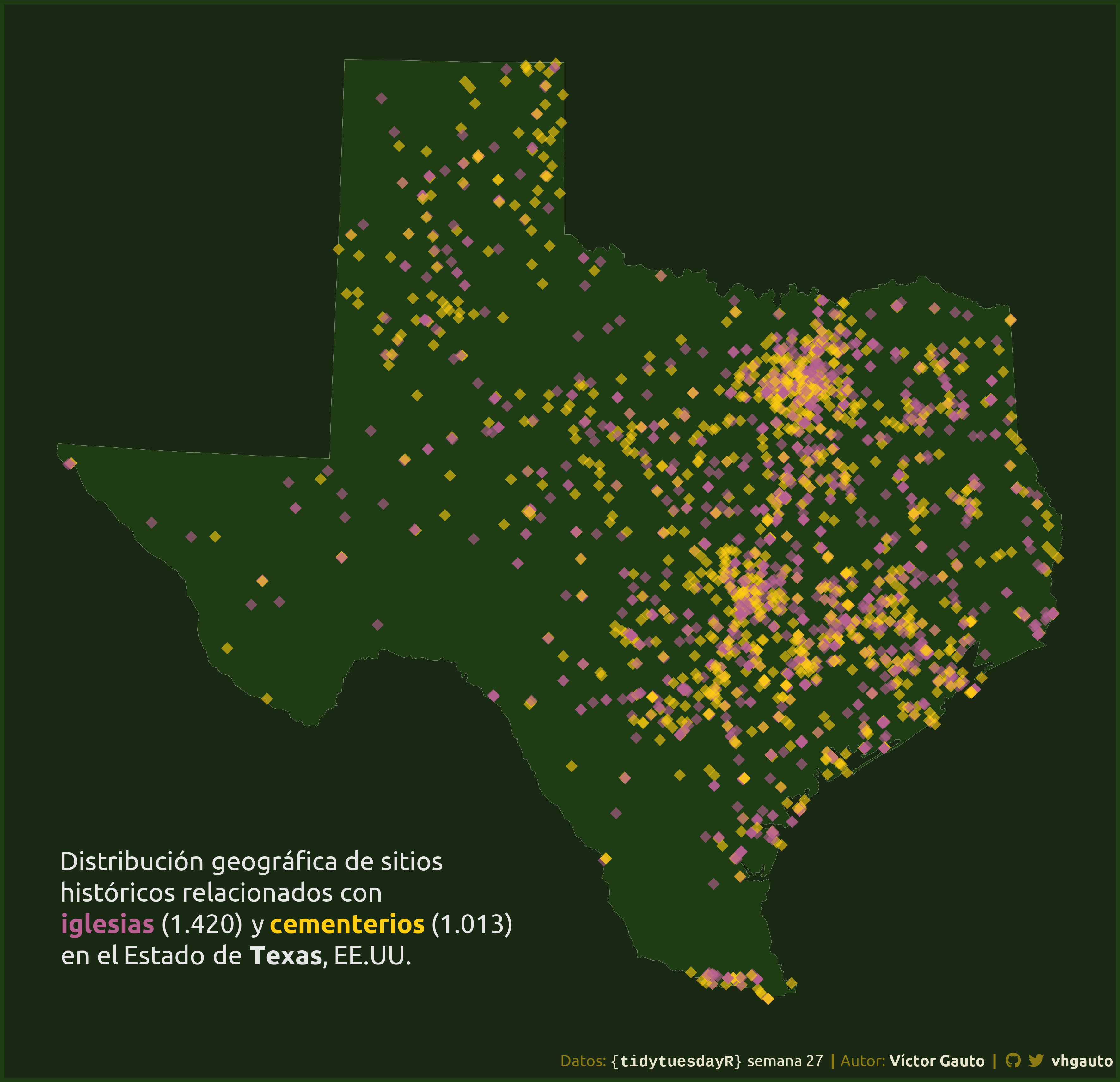
    "Distribución geográfica de sitios<br>
    históricos relacionados con<br>
    <span style='color:#B86092;'>**iglesias**</span> ({n_iglesia}) y 
    <span style='color:#FFCD11;'>**cementerios**</span> ({n_cementerio})<br>
    en el Estado de **Texas**, EE.UU."))

# figura
g <- ggplot() +
  geom_sf(data = texas, fill = c2, color = c3, linewidth = .05) +
  geom_sf(
    data = d, aes(color = sitio), 
    size = 4, alpha = .6, show.legend = FALSE, shape = 18) +
  geom_richtext(
    data = texto, aes(x = x, y = y, label = label),
    color = "grey90", label.color = NA, fill = NA, size = 7, hjust = 0,
    family = "ubuntu") +
  scale_color_manual(values = c(c4, c5)) +
  labs(caption = mi_caption) +
  theme_void() +
  theme(
    # plot.margin = margin(8, 5, 8, 5),
    plot.margin = margin(9.3, 5, 9.3, 5),
    plot.background = element_rect(fill = c1, color = c2, linewidth = 3),
    plot.caption = element_markdown(size = 12, color = c4, family = "ubuntu")
  )

# guardo
ggsave(
    plot = g,
    filename = "2023/semana_27/viz.png",
    width = 30, 
    height = 29,
    units = "cm",
    dpi = 300
  )

# abro
browseURL("2023/semana_27/viz.png")
Figura

Subir