Ocultar código
library(glue)
library(ggtext)
library(showtext)
library(tidyterra)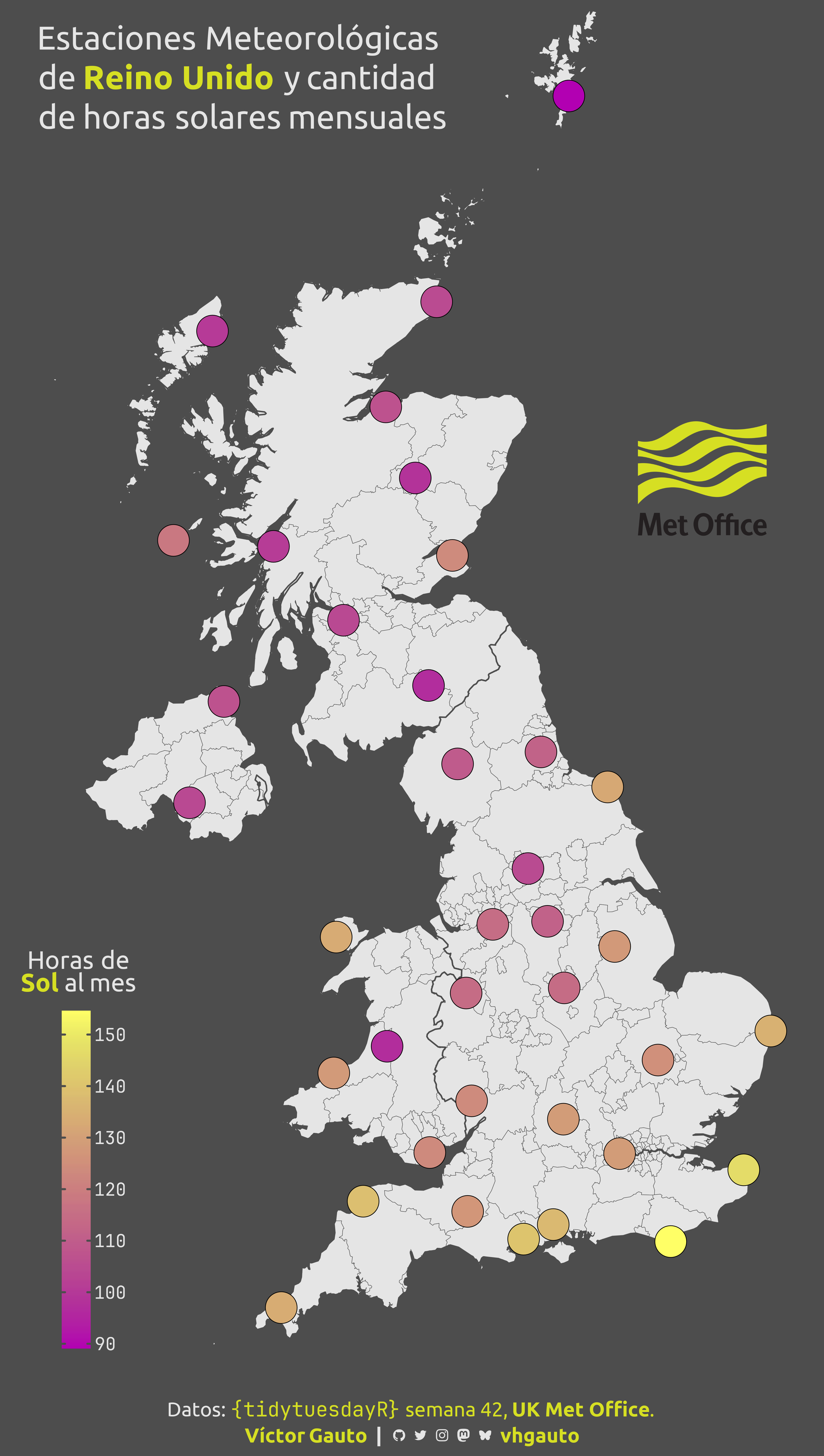
library(tidyverse)Estaciones meteorológicas de Reino Unido y cantidad de horas de Sol.
library(glue)
library(ggtext)
library(showtext)
library(tidyterra)
library(tidyverse)Colores.
c1 <- "grey30"
c2 <- "grey90"
c3 <- "black"
c4 <- "#D6DF23"
Fuentes: Ubuntu y JetBrains Mono.
font_add(
  family = "ubuntu",
  regular = "././fuente/Ubuntu-Regular.ttf",
  bold = "././fuente/Ubuntu-Bold.ttf",
  italic = "././fuente/Ubuntu-Italic.ttf"
)

font_add(
  family = "jet",
  regular = "././fuente/JetBrainsMonoNLNerdFontMono-Regular.ttf"
)

showtext_auto()
showtext_opts(dpi = 300)fuente <- glue(
"Datos: <span style='color:{c4};'><span style='font-family:jet;'>",
"{{<b>tidytuesdayR</b>}}</span> semana 42, ",
"<b>UK Met Office</b>.</span>"
)
autor <- glue("<span style='color:{c4};'>**Víctor Gauto**</span>")
icon_twitter <- glue("<span style='font-family:jet;'></span>")
icon_instagram <- glue("<span style='font-family:jet;'></span>")
icon_github <- glue("<span style='font-family:jet;'></span>")
icon_mastodon <- glue("<span style='font-family:jet;'>󰫑</span>")
icon_bsky <- glue("<span style='font-family:jet;'></span>")
usuario <- glue("<span style='color:{c4};'>**vhgauto**</span>")
sep <- glue("**|**")
mi_caption <- glue(
"{fuente}<br>{autor} {sep} {icon_github} {icon_twitter} {icon_instagram} ",
"{icon_mastodon} {icon_bsky} {usuario}"
)tuesdata <- tidytuesdayR::tt_load(2025, 42)
historic_station_met <- tuesdata$historic_station_met
station_meta <- tuesdata$station_metaMe interesa indicar los sitios de las estaciones meteorológicas y la cantidad de horas solares.
p <- terra::vect(station_meta, geom = c("lng", "lat"), crs = "EPSG:4326")Obtengo las fronteras de Reino Unido y condados.
uk1 <- rgeoboundaries::gb_adm1(country = "GBR") |>
  terra::vect()

uk2 <- rgeoboundaries::gb_adm2(country = "GBR") |>
  terra::vect()
Calculo la cantidad promedio de horas solares en cada estación meteorológica.
v <- historic_station_met |>
  reframe(
    m = mean(sun, na.rm = TRUE),
    .by = station
  ) |>
  inner_join(terra::as.data.frame(p, geom = "xy"), by = join_by(station)) |>
terra::vect(geom = c("x", "y"), crs = "EPSG:4326")Título de la figura, título de la leyenda y logo.
mi_titulo <- glue(
  "Estaciones Meteorológicas<br>de <b style='color: {c4};'>Reino Unido</b> ",
  "y cantidad<br>de horas solares mensuales"
)

mi_leyenda <- glue("Horas de<br><b style='color: {c4}'>Sol</b> al mes")

logo_tbl <- tibble(
  image = "https://upload.wikimedia.org/wikipedia/en/thumb/f/f4/Met_Office.svg/768px-Met_Office.svg.png",
  x = I(.9),
  y = I(.65)
)
Figura.
g <- ggplot() +
  geom_spatvector(
    data = uk2,
    alpha = 1,
    fill = c2,
    color = c1,
    linewidth = .2,
    show.legend = FALSE
  ) +
  geom_spatvector(data = uk1, fill = NA, linewidth = .7, color = c1) +
  geom_spatvector(
    data = v,
    aes(fill = m),
    size = 15,
    shape = 21,
    color = c3
  ) +
  ggimage::geom_image(
    data = logo_tbl,
    aes(x, y, image = image),
    inherit.aes = FALSE,
    size = .1
  ) +
  annotate(
    geom = "richtext",
    x = I(-.02),
    y = I(.99),
    label = mi_titulo,
    family = "ubuntu",
    size = 12,
    color = c2,
    hjust = 0,
    vjust = 1,
    fill = NA,
    label.color = NA
  ) +
  scico::scale_fill_scico(palette = "buda", breaks = scales::breaks_width(10)) +
  coord_sf(expand = FALSE, clip = "off") +
  labs(
    fill = mi_leyenda,
    caption = mi_caption
  ) +
  theme_void(base_size = 26, base_family = "ubuntu") +
  theme(
    plot.background = element_rect(fill = c1),
    plot.margin = margin(t = 10, b = 10),
    plot.caption = element_markdown(
      color = c2,
      hjust = .5,
      lineheight = 1.3,
      margin = margin(t = 55)
    ),
    legend.position = "inside",
    legend.position.inside = c(0, 0),
    legend.justification.inside = c(0, 0),
    legend.title = element_markdown(
      margin = margin(b = 15, l = -30),
      color = c2,
      hjust = .5
    ),
    legend.text = element_text(
      family = "jet",
      size = rel(.7),
      margin = margin(l = 5),
      color = c2
    ),
    legend.key.width = unit(30, "pt"),
    legend.key.height = unit(70, "pt"),
    legend.box.spacing = unit(0, "pt"),
    legend.ticks = element_line(linewidth = 1, color = c1)
  )
Guardo.
ggsave(
  plot = g,
  filename = "tidytuesday/2025/semana_42.png",
  width = 30,
  height = 53,
  units = "cm"
)