Ocultar código
library(glue)
library(ggtext)
library(showtext)
library(tidyverse)Canciones repetidas en el Billboard Hot 100.
library(glue)
library(ggtext)
library(showtext)
library(tidyverse)Colores.
c1 <- "#FFB3B5"
c2 <- "#7D0112"
# c3 <- "#4B1D91"
c3 <- "#310048"
c4 <- "#D3D9FF"
Fuentes: Ubuntu y JetBrains Mono.
font_add(
  family = "ubuntu",
  regular = "././fuente/Ubuntu-Regular.ttf",
  bold = "././fuente/Ubuntu-Bold.ttf",
  italic = "././fuente/Ubuntu-Italic.ttf"
)

font_add(
  family = "jet",
  regular = "././fuente/JetBrainsMonoNLNerdFontMono-Regular.ttf"
)

font_add(
  family = "bebas",
  regular = "././fuente/BebasNeue-Regular.ttf"
)

showtext_auto()
showtext_opts(dpi = 300)fuente <- glue(
"Datos: <span style='color:{c3};'><span style='font-family:jet;'>",
"{{<b>tidytuesdayR</b>}}</span> semana 34, ",
"<b>Billboard Hot 100 Number Ones Database</b>.</span>"
)
autor <- glue("<span style='color:{c3};'>**Víctor Gauto**</span>")
icon_twitter <- glue("<span style='font-family:jet;'></span>")
icon_instagram <- glue("<span style='font-family:jet;'></span>")
icon_github <- glue("<span style='font-family:jet;'></span>")
icon_mastodon <- glue("<span style='font-family:jet;'>󰫑</span>")
icon_bsky <- glue("<span style='font-family:jet;'></span>")
usuario <- glue("<span style='color:{c3};'>**vhgauto**</span>")
sep <- glue("**|**")
mi_caption <- glue(
"{fuente}<br>{autor} {sep} {icon_github} {icon_twitter} {icon_instagram} ",
"{icon_mastodon} {icon_bsky} {usuario}"
)tuesdata <- tidytuesdayR::tt_load(2025, 34)
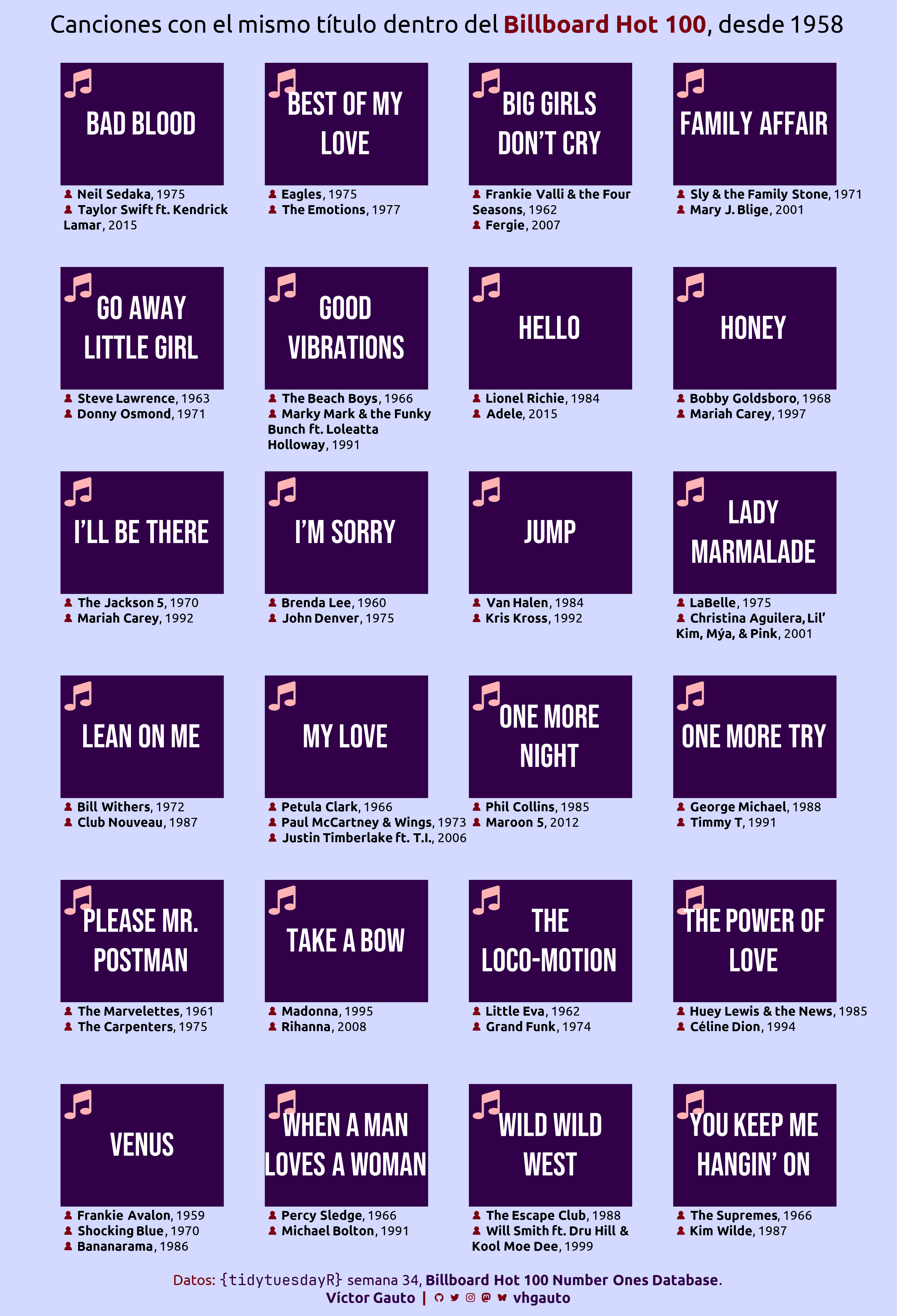
billboard <- tuesdata$billboardMe interesan las canciones con el mismo nombre, indicando los artistas y el año.
Canciones repetidas.
s <- billboard |>
  count(song, sort = TRUE) |>
  filter(n >= 2) |>
  pull(song)
Defino la cantidad de elementos a lo ancho y alto. Agrego íconos para las etiquetas de texto para la figura.
ancho_song <- 4
alto_song <- 6
icon_music <- glue(
"<span style='font-family:jet; color: {c1};'></span>"
)
icon_artist <- glue(
"<span style='font-family:jet; color: {c2};'></span>"
)Filtro los datos por las canciones seleccionadas y genero las etiquetas incorporando los íconos.
d <- billboard |>
  filter(song %in% s) |>
  mutate(año = year(date)) |>
  select(song, artist, año) |>
  arrange(song, año) |>
  mutate(artist = str_wrap(artist, 26)) |>
  mutate(artist = str_replace_all(artist, "\n", "<br>")) |>
  mutate(artista_año = glue("{icon_artist} <b>{artist}</b>, {año}")) |>
  nest(.by = song) |>
  mutate(
    label = map_chr(data, ~ str_flatten(.x$artista_año, collapse = "<br>"))
  ) %>%
  mutate(x = rep(1:ancho_song, length.out = nrow(.))) %>%
  mutate(y = rep(alto_song:1, each = ancho_song, length.out = nrow(.))) |>
  mutate(song = str_wrap(song, 13)) |>
mutate(song = str_replace_all(song, "\n", "<br>"))Ancho y alto del recuadro detrás de los nombres de las canciones y el título de la figura.
ancho_art <- .8
alto_art <- .6

mi_titulo <- glue(
  "Canciones con el mismo título dentro del <b style='color: {c2};'>Billboard Hot 100</b>, desde
  {year(min(billboard$date))}"
)
Figura.
g <- ggplot(d, aes(x, y)) +
  geom_tile(width = ancho_art, height = alto_art, fill = c3) +
  geom_richtext(
    aes(label = icon_music, x = x - ancho_art / 2, y = y + alto_art / 2),
    fill = NA,
    hjust = 0,
    vjust = 1,
    size = 15,
    label.color = NA
  ) +
  geom_richtext(
    aes(label = song),
    size = 11,
    family = "bebas",
    fill = NA,
    label.color = NA,
    color = "white"
  ) +
  geom_richtext(
    aes(x = x - ancho_art / 2, y = y - alto_art / 2, label = label),
    size = 4.3,
    fill = NA,
    label.color = NA,
    family = "ubuntu",
    hjust = 0,
    vjust = 1,
    color = "black"
  ) +
  coord_equal(clip = "off") +
  labs(title = mi_titulo, caption = mi_caption) +
  theme_void(base_family = "ubuntu", base_size = 10) +
  theme(
    plot.background = element_rect(fill = c4, color = NA),
    plot.title = element_markdown(
      size = rel(2.3),
      hjust = .5,
      margin = margin(t = 15, b = -30)
    ),
    plot.caption = element_markdown(
      color = c2,
      size = rel(1.4),
      lineheight = 1.2,
      hjust = .5,
      margin = margin(b = 10, t = 10)
    )
  )
Guardo.
ggsave(
  plot = g,
  filename = "tidytuesday/2025/semana_34.png",
  width = 30,
  height = 44,
  units = "cm"
)