Semana 07

Figura semana 07

Consumos durante San Valentín y cambio en el porcentaje de personas que participan.

Script

# paquetes ----------------------------------------------------------------

library(glue)
library(ggtext)
library(showtext)
library(patchwork)
library(tidyverse)

# fuente ------------------------------------------------------------------

# colores
c1 <- "black"
c2 <- "red"
c3 <- alpha("red", .6)
c4 <- "white"

# fuente: Ubuntu
font_add(
  family = "ubuntu", 
  regular = "fuente/Ubuntu-Regular.ttf",
  bold = "fuente/Ubuntu-Bold.ttf",
  italic = "fuente/Ubuntu-Italic.ttf")

# fuente: Victor
font_add(
  family = "victor", 
  regular = "fuente/VictorMono-ExtraLight.ttf",
  bold = "fuente/VictorMono-VariableFont_wght.ttf",
  italic = "fuente/VictorMono-ExtraLightItalic.ttf")

# fuente: Bebas Neue
font_add(
  family = "bebas", 
  regular = "fuente/BebasNeue-Regular.ttf")

# título
font_add_google(
  name = "Metamorphous",
  family = "metamorphous")

# íconos
font_add("fa-brands", "icon/Font Awesome 6 Brands-Regular-400.otf")

showtext_auto()
showtext_opts(dpi = 300)

# caption
fuente <- glue(
  "Datos: <span style='color:{c2};'><span style='font-family:mono;'>",
  "{{<b>tidytuesdayR</b>}}</span> semana {7}. ",
  "National Retail Federation.</span>")
autor <- glue("<span style='color:{c2};'>**Víctor Gauto**</span>")
icon_twitter <- glue("<span style='font-family:fa-brands;'>&#xf099;</span>")
icon_github <- glue("<span style='font-family:fa-brands;'>&#xf09b;</span>")
icon_mastodon <- glue("<span style='font-family:fa-brands;'>&#xf4f6;</span>")
usuario <- glue("<span style='color:{c2};'>**vhgauto**</span>")
sep <- glue("**|**")
dolar <- glue("<span style='color:{c2};'>**$** = USD</span>")

mi_caption <- glue(
  "{dolar} {sep} {fuente}<br>{autor} {sep} {icon_github} {icon_twitter} 
  {icon_mastodon} {usuario}")

# datos -------------------------------------------------------------------

tuesdata <- tidytuesdayR::tt_load(2024, 7)
historical_spending <- tuesdata$historical_spending

# me interesa ver la evolución de dinero dedicado a cada producto, y el 
# porcentaje de personas que festeja San Valentín

# categorías, vector en inglés
cc_vec <- historical_spending |> 
  janitor::clean_names() |> 
  pivot_longer(
    cols = -year,
    names_to = "categ",
    values_to = "valor"
  ) |> 
  rename(año = year) |> 
  distinct(categ) |> 
  pull()

# reordeno las categorías
cc_vec <- c(cc_vec[2:5], cc_vec[1], cc_vec[6:9])

# traducción de las categorías
cc_trad <- c(
  "Por persona", "Golosinas", "Flores", "Joyas", 
  "Personas que festejannSan Valentín",
  "Tarjeta de felicitaciones", "Salida de noche", "Ropa",
  "Tarjeta de regalos")

names(cc_trad) <- cc_vec

# agrego las traducciones y cambio a tabla larga
d <- historical_spending |> 
  janitor::clean_names() |> 
  pivot_longer(
    cols = -year,
    names_to = "categ",
    values_to = "valor"
  ) |> 
  rename(año = year) |> 
  mutate(cate = cc_trad[categ]) |> 
  select(-categ)

# figura ------------------------------------------------------------------

# eje vertical, por categoría
eje_y <- list(
  "Personas que festejannSan Valentín" = 
    scale_y_continuous(
      limits = c(50, 62), breaks = seq(50, 62, 2),
      labels = scales::label_number(suffix = "%")),
  "Por persona" =
    scale_y_continuous(
      limits = c(100, 200), breaks = seq(100, 200, 25),
      labels = scales::label_dollar()),
  "Golosinas" =
    scale_y_continuous(
      limits = c(5, 20), breaks = seq(5, 20, 5), 
      labels = scales::label_dollar()),
  "Flores" =
    scale_y_continuous(
      limits = c(12, 18), breaks = seq(12, 18, 1),
      labels = scales::label_dollar()),
  "Joyas" = 
    scale_y_continuous(
      limits = c(20, 50), breaks = seq(20, 50, 5), 
      labels = scales::label_dollar()),
  "Tarjeta de felicitaciones" =
    scale_y_continuous(
      limits = c(5, 10), breaks = seq(5, 10, 1), 
      labels = scales::label_dollar()),
  "Salida de noche" =
    scale_y_continuous(
      limits = c(20, 35), breaks = seq(20, 35, 5), 
      labels = scales::label_dollar()),
  "Ropa" =
    scale_y_continuous(
      limits = c(10, 25), breaks = seq(10, 25, 5), 
      labels = scales::label_dollar()),
  "Tarjeta de regalos" = 
    scale_y_continuous(
      limits = c(5, 20), breaks = seq(5, 20, 5), 
      labels = scales::label_dollar())
)

# colores, por categoría
# elimino un color, amarillento, no queda bien en la figura final
paleta_colores <- MoMAColors::moma.colors(palette_name = "Klein", n = 10)

co <- paleta_colores[paleta_colores != "#f9c000"]
names(co) <- cc_trad

# colores de fondo, por categoría
co2 <- c(
  "#FFEDF0", "#EEF5F6", "#FCF1E7", "#F3F7EA", "#000000", "#F2F7F3", "#F2E8EA",
  "#EAE9ED", "#F9EAE6"
)
names(co2) <- cc_trad

# título y subtítulo
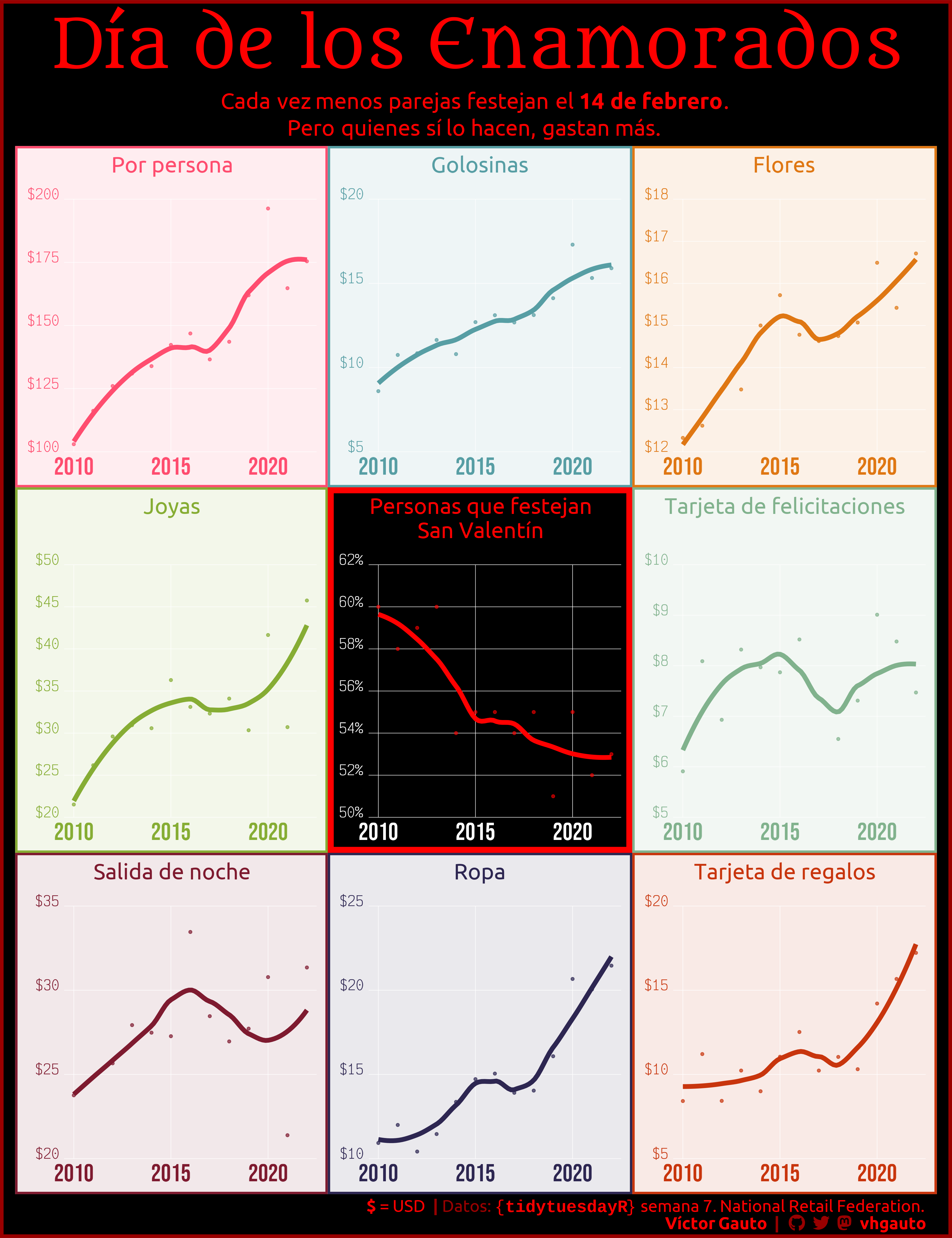
mi_title <- "Día de los Enamorados"
mi_subtitle <- glue(
  "Cada vez menos parejas festejan el **14 de febrero**.<br>",
  "Pero quienes sí lo hacen, gastan más."
)

# función que genera una figura p/c categoría
# el cambio en el tiempo de personas que festejan San Valentín tiene un color
# diferente del resto, y se ubica en el medio
f_gg <- function(x) {
  
  # datos filtrados
  tbl <- filter(d, cate == x)
  
  # eje vertical
  eje_y_break <- eje_y[[x]]
  
  # colores y ancho de línea del contorno
  color_fondo <- co2[x]
  color_linea <- co[x]
  color_eje <- co[x]
  color_titulo <- co[x]
  color_punto <- alpha(co[x], .7)
  color_borde <- co[x]
  linea <- 2
  
  # específicos de esta categoría
  if (x == "Personas que festejannSan Valentín") {
    color_fondo <- c1
    color_linea <- c2
    color_eje <- c4
    color_titulo <- c2
    color_punto <- c3
    color_borde <- c2
    linea <- 5
  }
  
  # figura
  g <- ggplot(tbl, aes(año, valor)) +
    geom_smooth(
      se = FALSE, formula = y ~ x, method = loess, color = color_linea,
      linewidth = 2) +
    geom_point(color = color_punto, size = 1, shape = 19) +
    scale_x_continuous(
      labels = c(2010, 2015, 2020), 
      breaks = c(2010, 2015, 2020), 
      limits = c(2009.5, 2022.5)) +
    eje_y_break +
    coord_cartesian(clip = "off", expand = FALSE) +
    labs(x = NULL, y = NULL, title = x) +
    theme_minimal() +
    theme(
      aspect.ratio = 1,
      plot.margin = margin(10, 10, 10, 10),
      plot.background = element_rect(
        fill = color_fondo, color = color_borde, linewidth = linea),
      plot.title.position = "plot",
      plot.title = element_text(
          family = "ubuntu", color = color_titulo, margin = margin(b = 20),
          size = 20, hjust = .5),
      panel.grid.minor = element_blank(),
      panel.grid.major = element_line(linewidth = .2, color = c4),
      axis.text.x = element_text(
        family = "bebas", color = color_eje, size = 22),
      axis.text.y = element_text(
        family = "victor", color = color_eje, vjust = 0, size = 12)
    )
  
  return(g)
}

# lista con todas las figuras
gg_lista <- map(cc_trad, f_gg)

# figura
g <- wrap_plots(gg_lista, ncol = 3) +
  plot_annotation(
    title = mi_title,
    subtitle = mi_subtitle,
    caption = mi_caption,
    theme = theme(
      plot.margin = margin(t = 15, r = 13.6, l = 13.6, b = 5),
      plot.background = element_rect(fill = c1, color = c3, linewidth = 3),
      plot.title = element_text(
        family = "metamorphous", size = 60, hjust = .5, color = c2),
      plot.subtitle = element_markdown(
        family = "ubuntu", size = 20, hjust = .5, color = c2, 
        lineheight = unit(1.2, "line")),
      plot.caption = element_markdown(family = "ubuntu", size = 15, color = c3),
      panel.background = element_rect(fill = c4)
    )
  )

# guardo
ggsave(
  plot = g,
  filename = "2024/s07/viz.png",
  width = 30,
  height = 39,
  units = "cm")

# abro
browseURL("2024/s07/viz.png")

Figura