Semana 45

Figura semana 45

Participación femenina en las elecciones de EE.UU.

Script

# paquetes ----------------------------------------------------------------

library(tidyverse)
library(fontawesome)
library(gender)
library(showtext)
library(glue)
library(ggtext)

# fuente ------------------------------------------------------------------

# colores
c1 <- "#88C0D0"
c2 <- "#81A1C1"
c3 <- "#5E81AC"
c4 <- "grey90"
c5 <- "#306489"
c6 <- "#222B4C"

# texto gral
font_add_google(name = "Ubuntu", family = "ubuntu")
# algoritmos, eje vertical
font_add_google(name = "Victor Mono", family = "victor", db_cache = FALSE)
# eje horizontal, años
font_add_google(name = "Bebas Neue", family = "bebas", db_cache = FALSE)
# título
font_add_google(name = "Vast Shadow", family = "vast")

# íconos
font_add("fa-brands", "icon/Font Awesome 6 Brands-Regular-400.otf")
font_add("fa-solids", "icon/Font Awesome 6 Free-Solid-900.otf")
font_add("fa-regular", "icon/Font Awesome 6 Free-Regular-400.otf")

showtext_auto()
showtext_opts(dpi = 300)

# caption
fuente <- glue(
  "Datos: <span style='color:{c3};'><span style='font-family:mono;'>",
  "{{<b>tidytuesdayR</b>}}</span> semana 45. ",
  "MIT Election Data and Science Lab, ",
  "**Harvard Dataverse**</span>")
autor <- glue("Autor: <span style='color:{c3};'>**Víctor Gauto**</span>")
icon_twitter <- glue("<span style='font-family:fa-brands;'>&#xf099;</span>")
icon_github <- glue("<span style='font-family:fa-brands;'>&#xf09b;</span>")
usuario <- glue("<span style='color:{c3};'>**vhgauto**</span>")
sep <- glue("**|**")

mi_caption <- glue(
  "{fuente}<br>{autor} {sep} {icon_github} {icon_twitter} {usuario}")

# datos -------------------------------------------------------------------

browseURL("https://github.com/rfordatascience/tidytuesday/blob/master/data/2023/2023-11-07/readme.md")

house <- readr::read_csv('https://raw.githubusercontent.com/rfordatascience/tidytuesday/master/data/2023/2023-11-07/house.csv')

# me interesa el género de los candidatos y la proporción en el tiempo

# función para obtener el 1er nombre, y si es una sola letra, el segundo
get_first_name <- function(name) {
  name_parts <- str_split(name, " ")[[1]]
  if (nchar(name_parts[1]) == 1) {
    return(name_parts[2])
  } else {
    return(name_parts[1])
  }
}

# primer nombre de cada candidato, agrupado por año
# se agrupan, por año, los mismos nombres
d <- house |> 
  filter(!writein) |> 
  select(year, candidate) |> 
  mutate(primer = map(.x = candidate, ~ get_first_name(name = .x))) |> 
  unnest(primer) |> 
  count(primer, .by = year) |> 
  arrange(.by) |> 
  rename(year = .by)

# por cada algoritmo, obtengo el género del candidato
d_ipums <- d |> 
  mutate(genero = map(
    .x = primer,
    (x) gender(x, countries = "United States", method = "ipums")$gender))

d_ssa <- d |> 
  mutate(genero = map(
    .x = primer,
    (x) gender(x, countries = "United States", method = "ssa")$gender))

d_napp <- d |> 
  mutate(genero = map(
    .x = primer,
    (x) gender(x, method = "napp")$gender))

# unifico los resultados de todos los algoritmos
e <- bind_rows(
  d_ipums |> mutate(tipo = "ipums"), 
  d_napp |> mutate(tipo = "napp"), 
  d_ssa |> mutate(tipo = "ssa")) |> 
  mutate(genero = as.character(genero)) |>
  filter(genero != "logical(0)") |>
  mutate(g = genero == "male") |>
  reframe(p = sum(g*n)/sum(n), .by = c(year, tipo)) |> 
  mutate(p = 1 - p)

# la asignación del género a partir del nombre, por cada algoritmo, lleva mucho
# tiempo. Entonces, guardo los resultados y leo desde el archivo .tsv
e |> 
  write_tsv("2023/semana_45/datos.tsv")

e <- read_tsv("2023/semana_45/datos.tsv")

# figura ------------------------------------------------------------------

# etiquetas de los algoritmos, para agregar en el borde derecho
algoritmo_label <- e |> 
  filter(year == max(e$year))

# función para aplicar fuente mono (victor) a los nombres de los algortimos
f_mono_it <- (x) glue("<span style='font-family:victor'>{x}</span>")

# puntos de la grilla, de fondo de la figura
p <- expand.grid(
  x = seq(1980, 2020, 10),
  y = seq(.1, .3, .05)) |> 
  as_tibble()

# título, subtítulo y aclaración del la asignación del género a partir de
# los algoritmos
mi_tit <- glue(
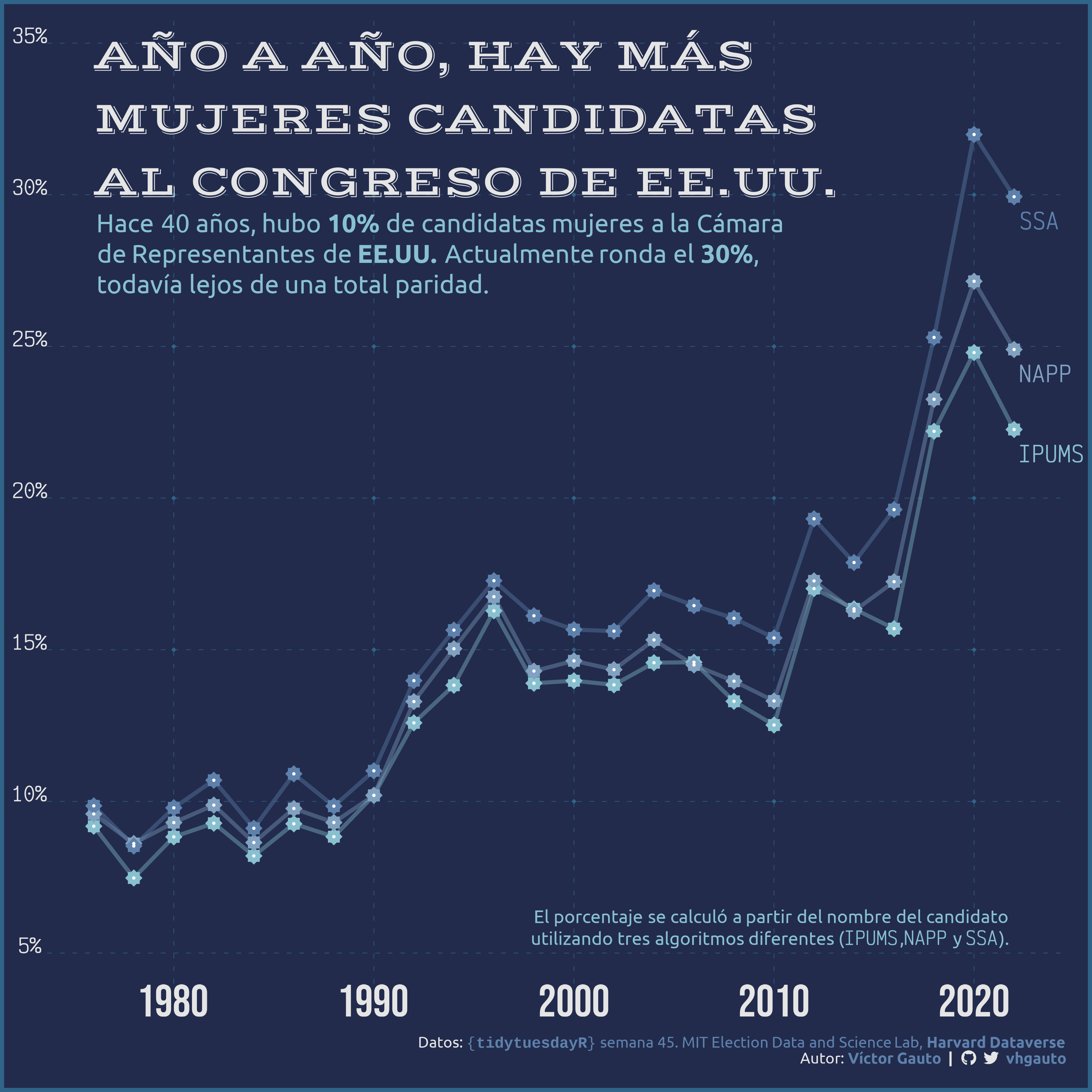
  "Año a año, hay másnmujeres candidatasnal Congreso de EE.UU.") |>
  str_to_upper()

mi_sub <- glue(
  "Hace 40 años, hubo **10%** de candidatas mujeres a la Cámara<br>",
  "de Representantes de **EE.UU.** Actualmente ronda el **30%**,<br>",
  "todavía lejos de una total paridad.<br>")

mi_texto <- glue(
  "El porcentaje se calculó a partir del nombre del candidato<br>",
  "utilizando tres algoritmos diferentes ({f_mono_it('IPUMS')},",
  "{f_mono_it('NAPP')} y {f_mono_it('SSA')}).")

# figura
g <- ggplot(e, aes(year, p, color = tipo)) +
  # puntos de la grilla
  annotate(geom = "point", x = p$x, y = p$y, color = c5, shape = 18) +
  # líneas de los algoritmos de género
  geom_line(alpha = .4, linewidth = 1.5, show.legend = FALSE) +
  # puntos
  geom_point(shape = 15, size = 4)  +
  geom_point(shape = 18, size = 6)  +
  geom_point(size = 1, color = "white", shape = 20) +
  # etiquetas de los algoritmos
  geom_text(
    data = algoritmo_label, aes(year, p, label = str_to_upper(tipo)), size = 6,
    hjust = 0, vjust = 1, nudge_x = .3, nudge_y = -.005, family = "victor")+
  # título
  annotate(
    geom = "text", x = 1976, y = .3, hjust = 0, vjust = 0, label = mi_tit, 
    family = "vast", size = 12, color = c4) +
  # subtítulo
  annotate(
    geom = "richtext", x = 1976, y = .295, hjust = 0, vjust = 1, label = mi_sub, 
    family = "ubuntu", size = 7, color = c1, fill = NA, label.color = NA) +
  # aclaración algoritmos
  annotate(
    geom = "richtext", x = 2022, y = .05, hjust = 1, vjust = 0, 
    label = mi_texto, family = "ubuntu", size = 5, color = c1, fill = NA, 
    label.color = NA) +
  scale_y_continuous(
    breaks = seq(.05, .35, .05), limits = c(.05, .35), expand = c(0, .01),
    labels = scales::label_percent(decimal.mark = ",", big.mark = ".")) +
  scale_color_manual(values = c(c1, c2, c3)) +
  coord_cartesian(clip = "off") +
  labs(caption = mi_caption) +
  theme_void() +
  theme(
    plot.margin = margin(10, 20, 10, 10),
    plot.background = element_rect(fill = c6, color = c5,linewidth = 3),
    plot.caption = element_markdown(
      color = c4, size = 12, family = "ubuntu", margin = margin(15, 0, 10, 0)),
    plot.caption.position = "plot",
    panel.grid.major = element_line(
      color = "#306489", linetype = "8f", linewidth = .2),
    axis.text = element_text(color = c4),
    axis.text.x = element_text(family = "bebas", size = 35),
    axis.text.y = element_text(family = "victor", size = 15, vjust = 0),
    legend.position = "none"
  )

# guardo
ggsave(
  plot = g,
  filename = "2023/semana_45/viz.png",
  width = 30,
  height = 30,
  units = "cm")

# abro
browseURL("2023/semana_45/viz.png")

Figura