# paquetes ----------------------------------------------------------------
library(tidyverse)
library(showtext)
library(here)
library(ggtext)
library(glue)
library(fontawesome)
library(sf)
library(patchwork)
library(ggrepel)
library(ggtext)
# fuentes -----------------------------------------------------------------
font_add_google(name = "Share Tech Mono", family = "share") # números
font_add_google(name = "Heebo", family = "heebo") # resto del texto
font_add_google(name = "Domine", family = "domine") # título
showtext_auto()
showtext_opts(dpi = 300)
# íconos
font_add("fa-reg", here("icon/Font Awesome 5 Free-Regular-400.otf"))
font_add("fa-brands", here("icon/Font Awesome 5 Brands-Regular-400.otf"))
font_add("fa-solid", here("icon/Font Awesome 5 Free-Solid-900.otf"))
# caption
icon_twitter <- "<span style='font-family:fa-brands; color:white;'></span>"
icon_github <- "<span style='font-family:fa-brands; color:white;'></span>"
fuente <- "<span style='color:white;'>Datos:</span> <span style='color:#16317d;'><span style='font-family:mono;'>{**tidytuesdayR**}</span> semana 13</span>"
autor <- "<span style='color:white;'>Autor:</span> <span style='color:#16317d;'>**Víctor Gauto**</span>"
sep <- glue("<span style = 'color:#a4cac8;'>**|**</span>")
usuario <- glue("<span style = 'color:#16317d;'>**vhgauto**</span>")
mi_caption <- glue("{fuente} {sep} {autor} {sep} {icon_github} {icon_twitter} {usuario}")
# datos -------------------------------------------------------------------
# browseURL("https://github.com/rfordatascience/tidytuesday/blob/master/data/2023/2023-03-28/readme.md")
# husos horarios
transitions <- readr::read_csv('https://raw.githubusercontent.com/rfordatascience/tidytuesday/master/data/2023/2023-03-28/transitions.csv')
timezones <- readr::read_csv('https://raw.githubusercontent.com/rfordatascience/tidytuesday/master/data/2023/2023-03-28/timezones.csv')
# mapa del mundo, p/obtener el CRS únicamente
# si uso 'crs = 4326' no queda igual, así que lo extraigo de 'world'
# world <- rnaturalearth::ne_countries(scale = "medium", returnclass = "sf")
# husos horarios Argentina
tz_arg_tbl <- timezones |>
filter(str_detect(zone, "Argentina")) |>
mutate(zone = str_remove(zone, "America/Argentina/"))
# convierto a 'sf', 4326
tz_arg <- st_as_sf(tz_arg_tbl, coords = c("longitude", "latitude"), crs = 4326)
# provincias argentinas
# descargado del Instituto Geográfico Nacional y convertido a .gpkg
# https://www.ign.gob.ar/NuestrasActividades/InformacionGeoespacial/CapasSIG
# 4326
pcias <- st_read(here("2023/semana_13/pcias.gpkg"))
# corrijo los nombres de las zonas
tz_arg <- tz_arg |>
mutate(zone = str_replace(zone, "_", " "))
# fechas de inicio/fin de horarios de verano
verano <- transitions |>
filter(str_detect(zone, "Argentina/Buenos_Aires")) |>
mutate(begin = as_datetime(begin),
end = as_datetime(end)) |>
select(-zone, -offset, -abbreviation) |>
mutate(inicio = as_date(begin),
fin = as_date(end)) |>
drop_na()
eje_y_lbl <- tibble(y = seq.Date(min(verano$inicio), ymd(20100101), "1 year")) |>
mutate(fecha = ymd(glue("{year(y)}0101"))) |>
mutate(año = year(fecha)) |>
mutate(decena = año %% 10 == 0) |>
mutate(label = if_else(decena == TRUE, glue("·{as.character(año)}"), "")) |>
mutate(largo = if_else(decena == TRUE, 3, 1))
# indicación 1er uso de horario de verano
verano_1 <- verano |>
filter(dst == TRUE) |>
slice(1) |>
mutate(label = glue("En {format(inicio, '%B')} de {year(inicio)}<br>fue la primera vez en<br>aplicarse horario de verano"))
# figuras -----------------------------------------------------------------
# mapa
g1 <- ggplot() +
# límites provinciales, borde grueso azul
geom_sf(data = pcias, color = "#16317d", fill = NA, linewidth = 1) +
# límites provinciales, borde fino amarillo
geom_sf(data = pcias, color = "#f6b40e", fill = NA, linewidth = .5) +
# ciudades
geom_sf(data = tz_arg, shape = 23, color = "white", fill = "#16317d",
size = 2) +
# etiquetas de las ciudades
geom_label_repel(data = tz_arg, aes(label = zone, geometry = geometry),
stat = "sf_coordinates", min.segment.length = Inf,
fill = alpha("#74acdf", .7), label.size = 0,
family = "heebo",
size = 5, color = "#16317d", force = 10, seed = 2023) +
# manual
coord_sf(clip = "on", ylim = c(-56, -21), xlim = c(-75, -50), expand = FALSE) +
# tema
theme_void() +
theme(plot.background = element_rect(fill = "#74acdf", color = NA),
panel.background = element_rect(fill = "#74acdf", color = NA))
# horarios de verano
g2 <- ggplot(data = verano,
aes(ymin = inicio, ymax = fin, xmin = 0, xmax = 1, fill = dst)) +
geom_rect() +
# borde
geom_rect(ymin = min(verano$inicio), ymax = max(verano$fin),
xmin = 0, xmax = 1, color = "#16317d", fill = NA) +
# 1er año
geom_richtext(data = verano_1, aes(x = -.1, y = inicio+months(12), label = label),
color = "#16317d", fill = NA, label.color = NA, size = 4,
hjust = 1, vjust = 1, family = "heebo") +
geom_text(data = verano_1, aes(x = -.1, y = inicio, label = "u25B6"),
color = "#16317d", size = 6) +
# manual
scale_y_date(sec.axis = sec_axis(trans = ~ .x,
breaks = eje_y_lbl$fecha,
labels = eje_y_lbl$label)) +
scale_fill_manual(values = c("#74acdf", "#f6b40e"),
breaks = c(TRUE, FALSE),
labels = c("Sí ", "No")) +
coord_cartesian(clip = "off", xlim = c(-1, 1),
ylim = c(ymd(18900101), ymd(20100101))) +
# ejes
labs(fill = "¿Fue año con horarionde verano?") +
# guía
guides(fill = guide_legend(override.aes = list(shape = 22,
color = "#16317d"))) +
theme(aspect.ratio = 7,
legend.position = c(.35, 0.03),
legend.spacing.x = unit(1, "line"),
legend.direction = "horizontal",
legend.title = element_text(family = "heebo", color = "#16317d", size = 12,
hjust = 1),
legend.text = element_text(color = "#16317d", family = "heebo", size = 12),
legend.key.width = unit(1.5, "line"),
legend.key.height = unit(1.5, "line"),
legend.background = element_rect(fill = "#74acdf", color = NA),
plot.margin = margin(0, 40, 0, 0),
plot.background = element_rect(fill = "#74acdf", color = NA),
panel.background = element_rect(fill = "#74acdf", color = NA),
panel.grid = element_blank(),
axis.title = element_blank(),
axis.text = element_blank(),
axis.ticks = element_blank(),
axis.ticks.length = unit(.3, "line"),
axis.ticks.y.right = element_line(color = "#16317d"),
axis.text.y.right = element_text(color = "white", size = 15,
family = "share", vjust = .45,
margin = margin(0, 0, 0, 3)))
# figura compuesta
g3 <- g1 + g2 &
plot_layout(widths = c(1, .25)) &
plot_annotation(
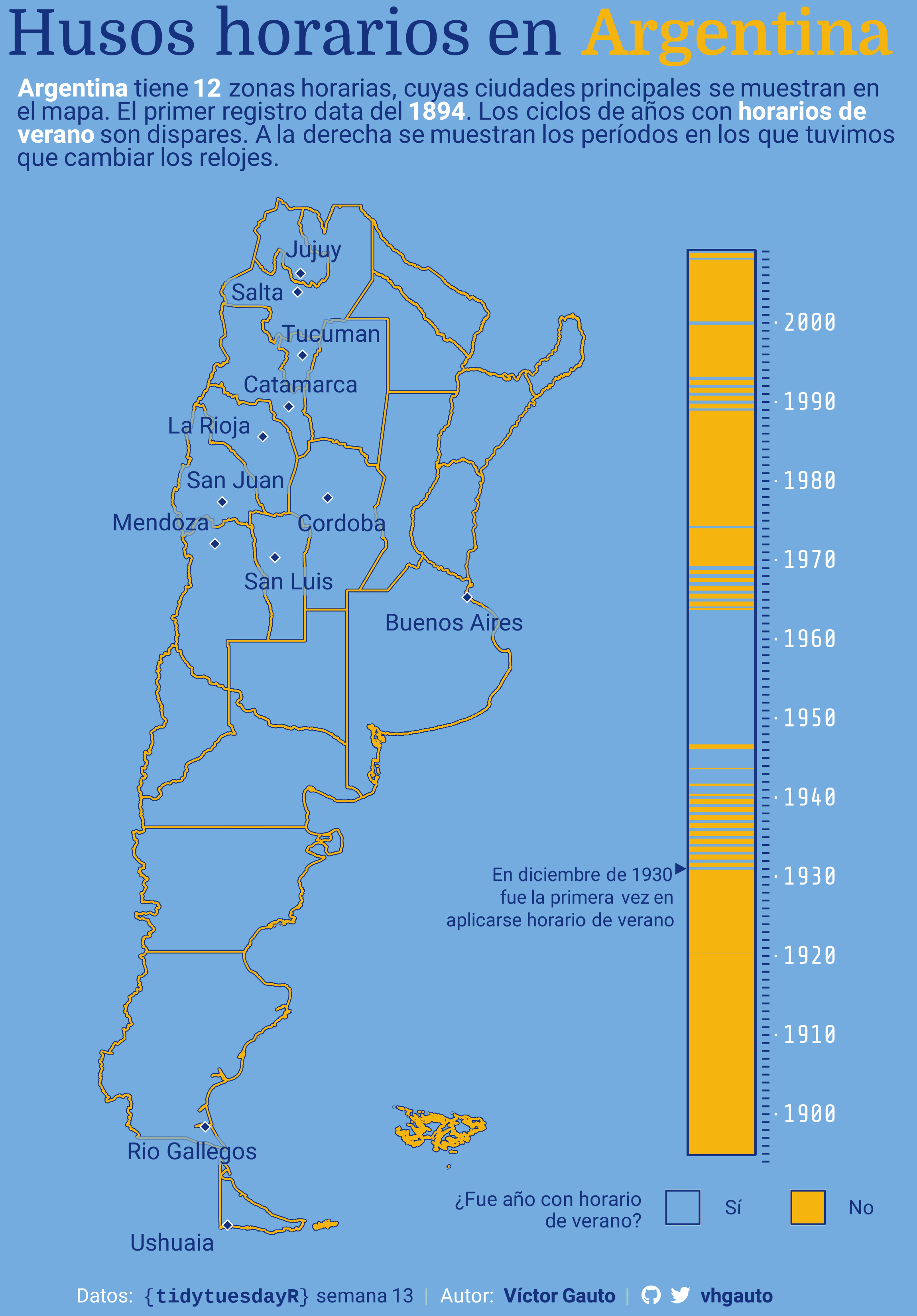
title = glue("Husos horarios en <span style='color:#f6b40e'>**Argentina**</span>"),
subtitle = glue("<span style='color:white'>**Argentina**</span> tiene
<span style='color:white'>**12**</span> zonas horarias,
cuyas ciudades principales se muestran en<br>el mapa. El
primer registro data del <span style='color:white'>**{year(min(verano$inicio))}**</span>.
Los ciclos de años con <span style='color:white'>**horarios de<br>verano**</span>
son dispares. A la derecha se muestran los períodos en los
que tuvimos<br>que cambiar los relojes."),
caption = mi_caption,
theme = theme(plot.background = element_rect(color = NA, fill = "#74acdf"),
plot.title.position = "plot",
plot.title = element_markdown(size = 38,
family = "domine",
color = "#16317d"),
plot.subtitle = element_markdown(color = "#16317d",
size = 15,
family = "heebo",
margin = margin(2, 0, 2, 5)),
plot.caption = element_markdown(hjust = .5,
family = "heebo",
margin = margin(10, 0, 0, 0),
size = 12),
plot.caption.position = "plot"))
# guardo
ggsave(plot = g3,
filename = here("2023/semana_13/viz.png"),
width = 2300,
height = 3300,
units = "px",
dpi = 300)
# abro
browseURL(here("2023/semana_13/viz.png"))