# paquetes ----------------------------------------------------------------
library(tidyverse)
library(ggwaffle)
library(glue)
library(ggtext)
library(showtext)
# fuentes -----------------------------------------------------------------
# colores, Renoir
c1 <- "#17164F"
c2 <- "#9D9CD5"
c3 <- "#6C5D9E"
c4 <- "#E69B00"
c5 <- "#BF3728"
c6 <- "#F6B3B0"
# texto gral
font_add_google(name = "Ubuntu", family = "ubuntu")
# título y porcentajes
font_add_google(name = "Victor Mono", family = "victor", db_cache = FALSE)
# íconos
font_add("fa-brands", "icon/Font Awesome 6 Brands-Regular-400.otf")
font_add("fa-solids", "icon/Font Awesome 6 Free-Solid-900.otf")
showtext_auto()
showtext_opts(dpi = 300)
# caption
fuente <- glue("Datos: <span style='color:{c3};'><span style='font-family:mono;'>{{<b>tidytuesdayR</b>}}</span> semana 29, **GPT Detectors Are Biased Against Non-Native English Writers**. Weixin Liang, Mert Yuksekgonul, Yining Mao, Eric Wu, James Zou. arXiv: **2304.02819**</span>")
autor <- glue("Autor: <span style='color:{c3};'>**Víctor Gauto**</span>")
icon_twitter <- glue("<span style='font-family:fa-brands;'></span>")
icon_github <- glue("<span style='font-family:fa-brands;'></span>")
usuario <- glue("<span style='color:{c3};'>**vhgauto**</span>")
sep <- glue("**|**")
mi_caption <- glue("{fuente}<br>{autor} {sep} {icon_github} {icon_twitter} {usuario}")
# datos -------------------------------------------------------------------
browseURL("https://github.com/rfordatascience/tidytuesday/blob/master/data/2023/2023-07-18/readme.md")
detectors <- readr::read_csv('https://raw.githubusercontent.com/rfordatascience/tidytuesday/master/data/2023/2023-07-18/detectors.csv')
# aciertos/errores en la detección de texto HUMANO
detectors |>
filter(kind == "Human") |>
summarise(acierto = mean(kind == .pred_class)) |>
mutate(error = 1 - acierto)
# aciertos/errores en la detección de texto IA
detectors |>
filter(kind == "AI") |>
summarise(acierto = mean(kind == .pred_class)) |>
mutate(error = 1 - acierto)
# aciertos/errores en la detección de texto HUMANO, entre nativos/NO nativos
detectors |>
filter(kind == "Human") |>
group_by(native) |>
summarise(acierto = mean(kind == .pred_class)) |>
mutate(error = 1 - acierto)
# porcentaje de aciertos entre texto generado por nativos del inglés
porc_nativo <- detectors |>
filter(kind == "Human" & native == "Yes") |>
summarise(acierto = mean(kind == .pred_class)) |>
pull(acierto) |>
gt::vec_fmt_percent(decimals = 0, sep_mark = ".", dec_mark = ",")
# porcentaje de aciertos entre texto generado por NO nativos del inglés
porc_no_nativo <- detectors |>
filter(kind == "Human" & native == "No") |>
summarise(acierto = mean(kind == .pred_class)) |>
pull(acierto) |>
gt::vec_fmt_percent(decimals = 0, sep_mark = ".", dec_mark = ",")
# me interesa el porcentaje de aciertos, entre nativos/NO nativos, para los
# siete detectores
d <- detectors |>
filter(!is.na(native)) |>
group_by(detector, native) |>
reframe(prop = mean(kind == .pred_class)) |>
mutate(detector = fct_reorder(detector, prop, max))
# figura ------------------------------------------------------------------
# título y subtítulo
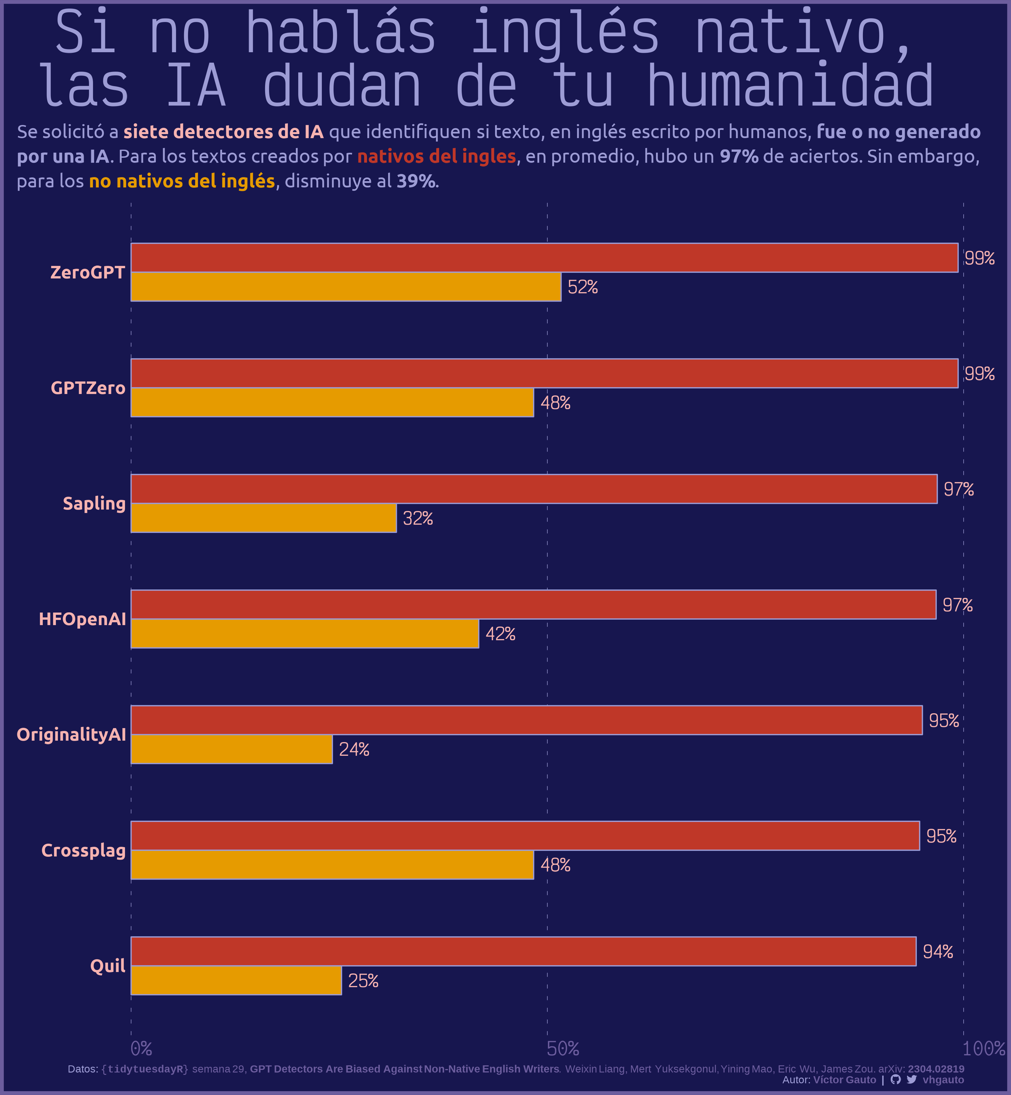
tit <- glue("Si no hablás inglés nativo,<br>las IA dudan de tu humanidad")
subtit <- glue(
"Se solicitó a <span style='color:{c6}'>**siete detectores de IA**</span> que
identifiquen si texto, en inglés escrito por humanos, **fue o no generado<br>
por una IA**. Para los textos creados por
<span style='color:{c5};'>**nativos del ingles**</span>, en promedio,
hubo un **{porc_nativo}** de aciertos. Sin embargo, <br>
para los <span style='color:{c4};'>**no nativos del inglés**</span>,
disminuye al **{porc_no_nativo}**."
)
# figura
g <- ggplot(data = d, aes(x = prop, y = detector, fill = native)) +
# columnas
geom_col(
position = position_dodge(), show.legend = FALSE, width = .5, color = c2) +
# porcentajes
geom_text(
aes(label = gt::vec_fmt_percent(
prop, decimals = 0, dec_mark = ",", sep_mark = ".")),
position = position_dodge(width = .5), color = c6, size = 5,
hjust = -.25, family = "victor") +
scale_x_continuous(
limits = c(0, 1), expand = c(0, 0), breaks = c(0, .5, 1),
labels = scales::label_percent()) +
scale_fill_manual(values = c(c4, c5)) +
labs(
x = NULL, y = NULL, title = tit, subtitle = subtit, caption = mi_caption) +
coord_cartesian(clip = "off") +
theme(
aspect.ratio = 1,
plot.background = element_rect(fill = c1, color = c3, linewidth = 3),
plot.margin = margin(8, 40, 8, 13),
plot.title.position = "plot",
plot.title = element_markdown(
color = c2, size = 45, family = "victor", hjust = .5),
plot.subtitle = element_markdown(
color = c2, family = "ubuntu", size = 16, margin = margin(2, 2, 10, 2),
lineheight = 1.3),
plot.caption = element_markdown(color = c2),
panel.background = element_blank(),
panel.grid = element_blank(),
panel.grid.major.x = element_line(
linewidth = .2, linetype = "8f", color = c2),
axis.text.y = element_text(
hjust = 1, color = c6, family = "ubuntu", size = 15,face = "bold"),
axis.text.x = element_text(
color = c3, size = 15, family = "victor", hjust = 0),
axis.ticks = element_blank()
)
# guardo
ggsave(
plot = g,
filename = "2023/semana_29/viz.png",
width = 30,
height = 32.5,
units = "cm"
)
# abro
browseURL("2023/semana_29/viz.png")