Semana 42

Figura semana 42

Identificar el cuadrante emocional de las canciones de Taylor Swift.

Script

# paquetes ----------------------------------------------------------------

library(tidyverse)
library(showtext)
library(glue)
library(ggtext)

# fuente ------------------------------------------------------------------

# colores
# scales::show_col(tayloRswift::swift_palettes$lover)
c1 <- "#76BAE0"
c2 <- "#0E3D5B"
c3 <- "#B8396B"
c4 <- "#FFD1D7"
c5 <- "grey10"

# texto gral
font_add_google(name = "Ubuntu", family = "ubuntu")
# ejes, explicaciones
font_add_google(name = "Victor Mono", family = "victor")
# esquina (sentimientos)
font_add_google(name = "Bebas Neue", family = "bebas")
# Taylor Swift
font_add_google(name = "Pattaya", family = "pattaya")

# íconos
font_add("fa-brands", "icon/Font Awesome 6 Brands-Regular-400.otf")
font_add("fa-solids", "icon/Font Awesome 6 Free-Solid-900.otf")

showtext_auto()
showtext_opts(dpi = 300)

# caption
fuente <- glue(
  "Datos: <span style='color:{c3};'><span style='font-family:mono;'>",
  "<b>{{tidytuesdayR}}</b></span> semana 42. ",
  "<span style='font-family:victor'>{{taylor}}</span>, ",
  "**W. Jake Thompson**</span>")
autor <- glue("Autor: <span style='color:{c3};'>**Víctor Gauto**</span>")
icon_twitter <- glue("<span style='font-family:fa-brands;'>&#xf099;</span>")
icon_github <- glue("<span style='font-family:fa-brands;'>&#xf09b;</span>")
usuario <- glue("<span style='color:{c3};'>**vhgauto**</span>")
sep <- glue("**|**")

mi_caption <- glue(
  "{fuente}<br>{autor} {sep} {icon_github} {icon_twitter} {usuario}")

# datos -------------------------------------------------------------------

browseURL("https://github.com/rfordatascience/tidytuesday/blob/master/data/2023/2023-10-17/readme.md")

taylor_all_songs <- readr::read_csv('https://raw.githubusercontent.com/rfordatascience/tidytuesday/master/data/2023/2023-10-17/taylor_all_songs.csv')

# origen de la idea del plano
browseURL("https://medium.com/@gregory2/visualizing-gorillaz-in-r-how-to-analyze-artists-using-spotifyr-ebae3e05491b")

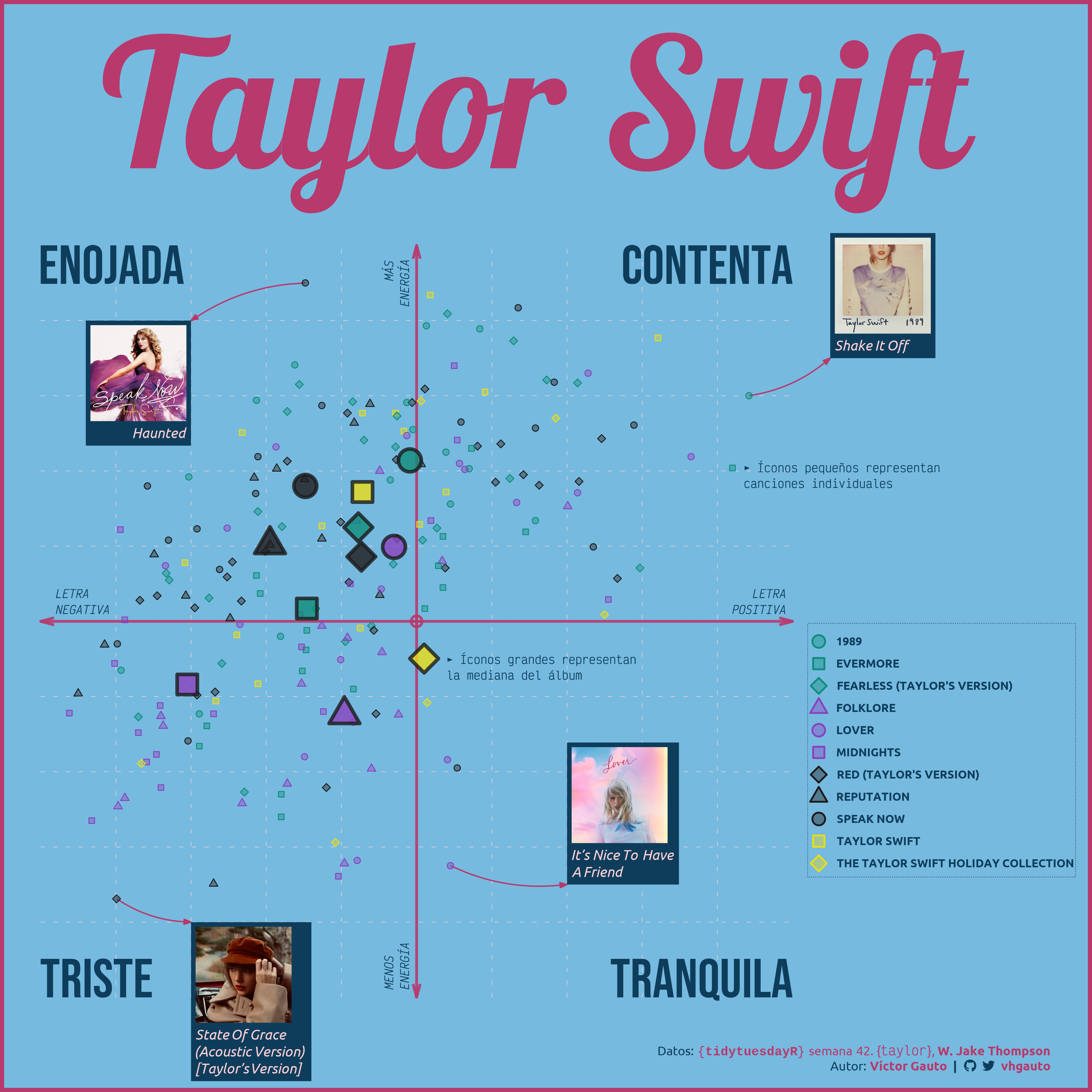
# me interesa analizar todas las canciones (que pertenezcan a algún álbum),
# de acuerdo a su valencia (positividad) y energía (intensidad/actividad)
# en base a esos dos parámetros, puedo establecer un plano de coordenadas
# que tiene en las esquinas cuatro sentimientos: enojo, felicidad, tristeza y
# tranquilidad

# explicación de c/feature
browseURL("https://developer.spotify.com/documentation/web-api/reference/get-several-audio-features")

# álbums que me interesan
album_tay <- c(
  "Taylor Swift", "Fearless (Taylor's Version)", "Speak Now", "1989", "evermore",
  "Red (Taylor's Version)", "reputation", "Lover", "folklore", "Midnights",
  "The Taylor Swift Holiday Collection")

# convierto el vector de nombres de álbum a factor
album_select <- taylor_all_songs |> 
  select(album_release, album_name) |> 
  filter(album_name %in% album_tay) |> 
  drop_na() |> 
  mutate(album_name = fct_reorder(album_name, album_release)) |> 
  mutate(album_name = fct_rev(album_name)) |> 
  distinct(album_name) |> 
  pull()

# todas las canciones
d <- taylor_all_songs |> 
  select(album_name, track_name, valence, energy) |> 
  filter(album_name %in% album_tay) |> 
  drop_na() |> 
  mutate(album_name = fct(album_name, levels = as.character(album_select))) |> 
  mutate(album_name = str_to_upper(album_name))

# canciones extremas de sentimientos
# calculo la distancia entre los puntos y el centro del cuadrante
# divido por cuadrante y obtengo un representante extremo por cada sentimiento
# contenta
d_contenta <- d |> 
  filter(between(valence, .5, 1) & between(energy, .5, 1)) |> 
  mutate(distancia = sqrt((valence - .5)^2 + (energy - .5)^2)) |> 
  slice_max(order_by = distancia, n = 1)

# enojada
d_enojada <- d |> 
  filter(between(valence, 0, .5) & between(energy, .5, 1)) |> 
  mutate(distancia = sqrt((valence - .5)^2 + (energy - .5)^2)) |> 
  slice_max(order_by = distancia, n = 1)

# triste
d_triste <- d |> 
  filter(between(valence, 0, .5) & between(energy, 0, .5)) |> 
  mutate(distancia = sqrt((valence - .5)^2 + (energy - .5)^2)) |> 
  slice_max(order_by = distancia, n = 1)

# tranquila
d_tranquila <- d |> 
  filter(between(valence, .5, 1) & between(energy, 0, .5)) |> 
  mutate(distancia = sqrt((valence - .5)^2 + (energy - .5)^2)) |> 
  slice_max(order_by = distancia, n = 1)

# sentimientos extremos
d_extremos <- bind_rows(d_contenta, d_enojada, d_triste, d_tranquila)

# figura ------------------------------------------------------------------

# paleta de colores para los puntos (canciones)
paleta <- MoMAColors::moma.colors(palette_name = "Fritsch")

# colores p/c álbum
album_color <- c(
  rep(paleta[1], 3),
  rep(paleta[2], 3),
  rep(paleta[3], 3),
  rep(paleta[4], 2))

# formas p/c álbum
album_shape <- rep(c(21, 22, 23, 24), 3)

# ejes en la mitad del plano
ejes_tbl <- tibble(
  x = c(0, .5), y = c(.5, 0), xend = c(1, .5), yend = c(.5, 1))

# grilla de líneas de trazos
grilla_v <- tibble(
  x = seq(.1, .9, .1), y = 0, xend = seq(.1, .9, .1), yend = 1)

# etiquetas de sentimientos en las esquinas del plano
sentimiento <- tibble(
  label = c("enojada", "contenta", "triste", "tranquila"),
  x = c(-Inf, Inf, -Inf, Inf),
  y = c(Inf, Inf, -Inf, -Inf),
  hjust = c(0, 1, 0, 1),
  vjust = c(1, 1, 0, 0))

# flechas, que unen tapas de álbum p/canciones extremas y los puntos
flechas_tbl <- tibble(
  x = d_extremos$valence*1,
  y = d_extremos$energy*1,
  xend = c(1.05, .2, .2, .7),
  yend = c(.85, .9, .1, .15))

# imágenes de las tapas de álbum
tapa_album <- list.files("2023/semana_42/", pattern = "ts", full.names = TRUE)

# etiqueta de las canciones extremas, con nombre de la canción y la tapa del
# álbum
img_album <- tibble(
  x = flechas_tbl$xend,
  y = flechas_tbl$yend,
  track = d_extremos$track_name,
  path = c(tapa_album[1], tapa_album[4], tapa_album[3], tapa_album[2])) |> 
  mutate(track = str_wrap(track, 18)) |> 
  mutate(track = str_replace_all(track, "\n", "<br>")) |> 
  mutate(label = glue(
    "<img src='{path}' width='75' /><br>",
    "<span style='font-family:ubuntu;'>*{track}*</span>")) |> 
  mutate(hjust = c(0, 1, 0, 0)) |> 
  mutate(vjust = c(0, 1, 1, 0))

# puntos que representan el álbum entero (mediana)
d_resumen <- d |> 
  summarise(
    valence = median(valence),
    energy = median(energy),
    .by = album_name)

# explicación de los ejes del plano
ejes_explic <- tibble(
  x = c(1, .5, .03, .5),
  y = c(.5, .97, .5, 0),
  label = c("LETRAnPOSITIVA", "MÁSnENERGÍA", "LETRAnNEGATIVA", "MENOSnENERGÍA"),
  angle = c(0, 90, 0, 90),
  hjust = c(1, 1, 0, 0),
  vjust = c(0, 0, 0, 0))

# explicación de los íconos pequeños/grandes
icono_grande <- "► Íconos grandes representannla mediana del álbum"
icono_peque <- "► Íconos pequeños representanncanciones individuales"

icono_tbl <- tibble(
  x = c(.54, .935),
  y = c(.455, .71),
  label = c(icono_grande, icono_peque))

# figura
g <- ggplot(d, aes(valence, energy)) +
  # grilla
  geom_vline(
    xintercept = seq(.1, .9, .1), color = c4, linetype = "8f", 
    linewidth = .2) +
  geom_hline(
    yintercept = seq(.1, .9, .1), color = c4, linetype = "8f", 
    linewidth = .2) +
  # etiqueta de las esquinas
  geom_text(
    data = sentimiento, aes(x, y, label = label, hjust = hjust, vjust = vjust),
    family = "bebas", size = 15, color = c2, inherit.aes = FALSE) +
  # ejes
  geom_segment(
    data = ejes_tbl, aes(x, y, xend = xend, yend = yend), inherit.aes = FALSE,
    color = c3, linewidth = 1, linetype = 1, alpha = .9,
    arrow = arrow(
      angle = 15, length = unit(.75, "line"), ends = "both", type = "open")) +
  # centro del plano
  annotate(
    geom = "point", x = .5, y = .5, size = 3, color = c3, shape = 10, 
    alpha = .9, stroke = 1.5) +
  # explicación de los íconos
  geom_text(
    data = icono_tbl, aes(x, y, label = label), inherit.aes = FALSE,
    color = c2, hjust = 0, vjust = 1, family = "victor", size = 3) +
  # explicación de los ejes del plano
  geom_text(
    data = ejes_explic, inherit.aes = FALSE,
    aes(x, y, label = label, angle = I(angle), hjust = hjust, vjust = vjust),
    family = "victor", fontface = "italic", size = 3, color = c2,
    nudge_x = -.01, nudge_y = .01) +
  # flechas
  geom_curve(
    data = flechas_tbl, aes(x, y, xend = xend, yend = yend), 
    inherit.aes = FALSE, curvature = .15, color = c3,
    arrow = arrow(angle = 20, length = unit(.4, "line"), type = "closed")) +
  # etiqueta de las canciones extremas
  geom_richtext(
    data = img_album, aes(x, y, label = label, hjust = hjust, vjust = vjust), 
    inherit.aes = FALSE, fill = c2, label.color = NA, 
    color = c4, label.r = unit(0, "line")) +
  # canciones individuales
  geom_point(
    aes(color = album_name, shape = album_name, fill = album_name), 
    size = 2, show.legend = TRUE, stroke = .5) +
  # álbums individuales (medianas)
  geom_point(data = d_resumen,
    aes(valence, energy, color = album_name, shape = album_name, 
        fill = album_name),
    size = 7, alpha = .8, show.legend = FALSE, stroke = 2, color = c5) +
  # caption
  annotate(
    geom = "richtext", x = 1.35, y = -.082, label = mi_caption, color = c2,
    family = "ubuntu", size = 3.5, hjust = 1, fill = NA, label.color = NA) +
  # manual
  scale_color_manual(values = album_color) +
  scale_fill_manual(values = alpha(album_color, .4)) +
  scale_shape_manual(values = album_shape) +
  coord_cartesian(
    xlim = c(0, 1), ylim = c(0, 1), expand = FALSE, clip = "off") +
  labs(
    x = NULL, y = NULL, color = NULL, shape = NULL, fill = NULL,
    title = "Taylor Swift") +
  guides(
    color = guide_legend(override.aes = list(size = 4, stroke = 1))) +
  theme_minimal() +
  theme(
    aspect.ratio = 1,
    plot.margin = margin(21.2, 234, 71.2, 29),
    plot.background = element_rect(
      fill = c1, color = c3, linewidth = 3),
    plot.title = element_text(
      family = "pattaya", color = c3, size = 140, hjust = -.5,
      margin = margin(5, 0, 25, 0)),
    plot.title.position = "panel",
    panel.grid = element_blank(),
    legend.text = element_text(family = "ubuntu", color = c2, face = "bold"),
    legend.background = element_rect(
      fill = c1, color = c2, linetype = 3, linewidth = .2),
    legend.position = c(1.02, .16),
    legend.margin = margin(0, 3, 2, 0),
    legend.justification = c(0, 0),
    axis.text = element_blank()
  )

# guardo
ggsave(
  plot = g,
  filename = "2023/semana_42/viz.png",
  width = 30,
  height = 30,
  units = "cm")

# abro
browseURL("2023/semana_42/viz.png")

Figura