# paquetes ----------------------------------------------------------------
library(glue)
library(ggtext)
library(showtext)
library(tidyverse)
# fuente ------------------------------------------------------------------
# colores
c1 <- "#040404"
c2 <- "#FCFCFC"
pal <- PrettyCols::prettycols(palette = "Light", n = 5)
# fuente: Ubuntu
font_add(
family = "ubuntu",
regular = "fuente/Ubuntu-Regular.ttf",
bold = "fuente/Ubuntu-Bold.ttf",
italic = "fuente/Ubuntu-Italic.ttf")
# monoespacio & íconos
font_add(
family = "jet",
regular = "fuente/JetBrainsMonoNLNerdFontMono-Regular.ttf")
showtext_auto()
showtext_opts(dpi = 300)
# caption
fuente <- glue(
"Datos: <span style='color:{pal[3]};'><span style='font-family:jet;'>",
"{{<b>tidytuesdayR</b>}}</span> semana {27}, ",
"<span style='font-family:jet;'>{{ttmeta}}</span>.</span>")
autor <- glue("<span style='color:{pal[3]};'>**Víctor Gauto**</span>")
icon_twitter <- glue("<span style='font-family:jet;'></span>")
icon_instagram <- glue("<span style='font-family:jet;'></span>")
icon_github <- glue("<span style='font-family:jet;'></span>")
icon_mastodon <- glue("<span style='font-family:jet;'>󰫑</span>")
usuario <- glue("<span style='color:{pal[3]};'>**vhgauto**</span>")
sep <- glue("**|**")
mi_caption <- glue(
"<span style='font-size:27px; color:{pal[5]}'>{fuente}<br>{autor} {sep} ",
"{icon_github} {icon_twitter} {icon_instagram} {icon_mastodon} ",
"{usuario}</span>")
# datos -------------------------------------------------------------------
tuesdata <- tidytuesdayR::tt_load(2024, 27)
tt_datasets <- tuesdata$tt_datasets
tt_variables <- tuesdata$tt_variables
# me interesan los datasets que incluyen variables geográficas
# y comparar con los otros datasets SIN datos geográficos
# filtro por datos geográficos
geo_tbl <- tt_variables |>
filter(
str_detect(variable, "^lat$|latitude|^lon$|longitude|lng|^long$|coord")
) |>
distinct(dataset_name, year, week) |>
arrange(year, week) |>
mutate(geo = "Con datos geográficos")
# combino los datos geográficos con el resto
d <- full_join(tt_datasets, geo_tbl, by = join_by(year, week, dataset_name)) |>
mutate(geo = if_else(is.na(geo), "Sin datos geográficos", geo)) |>
filter(geo == "Con datos geográficos") |>
select(year, week, geo)
# agrego los datos NO geográficos
e <- tt_datasets |>
distinct(year, week) |>
full_join(d, by = join_by(year, week)) |>
mutate(geo = if_else(is.na(geo), "Sin datos geográficos", geo))
# incluyo todas las semanas posibles
semanas_tbl <- expand_grid(
year = unique(tt_datasets$year),
week = unique(tt_datasets$week)) |>
arrange(year, week)
# última semana
max_dataset <- tt_datasets |>
filter(year == max(tt_datasets$year)) |>
slice_max(order_by = week, n = 1)
# combino todos los datos
e2 <- full_join(e, semanas_tbl, by = join_by(year, week)) |>
mutate(geo = if_else(is.na(geo), "Semana sin datos", geo)) |>
distinct() |>
arrange(year, week) |>
mutate(
estado = if_else(
year == max_dataset$year & week >= max_dataset$week,
"out",
"in"
)
) |>
filter(estado == "in")
# figura ------------------------------------------------------------------
# etiquetas del eje horizontal
eje_x_tbl <- unique(d$year) |>
str_split(pattern = "") |>
map(.x = _, ~ glue("{.x}<br>"))
eje_x_label <- tibble(eje_x_tbl) |>
mutate(label = map(.x = eje_x_tbl, str_flatten)) |>
unnest(label) |>
pull(label)
# cantidad de datos
n_datasets <- tt_datasets |>
distinct(year, week) |>
nrow()
n_geo <- e2 |>
filter(geo == "Con datos geográficos") |>
nrow()
# subtítulo
mi_subtitulo <- glue(
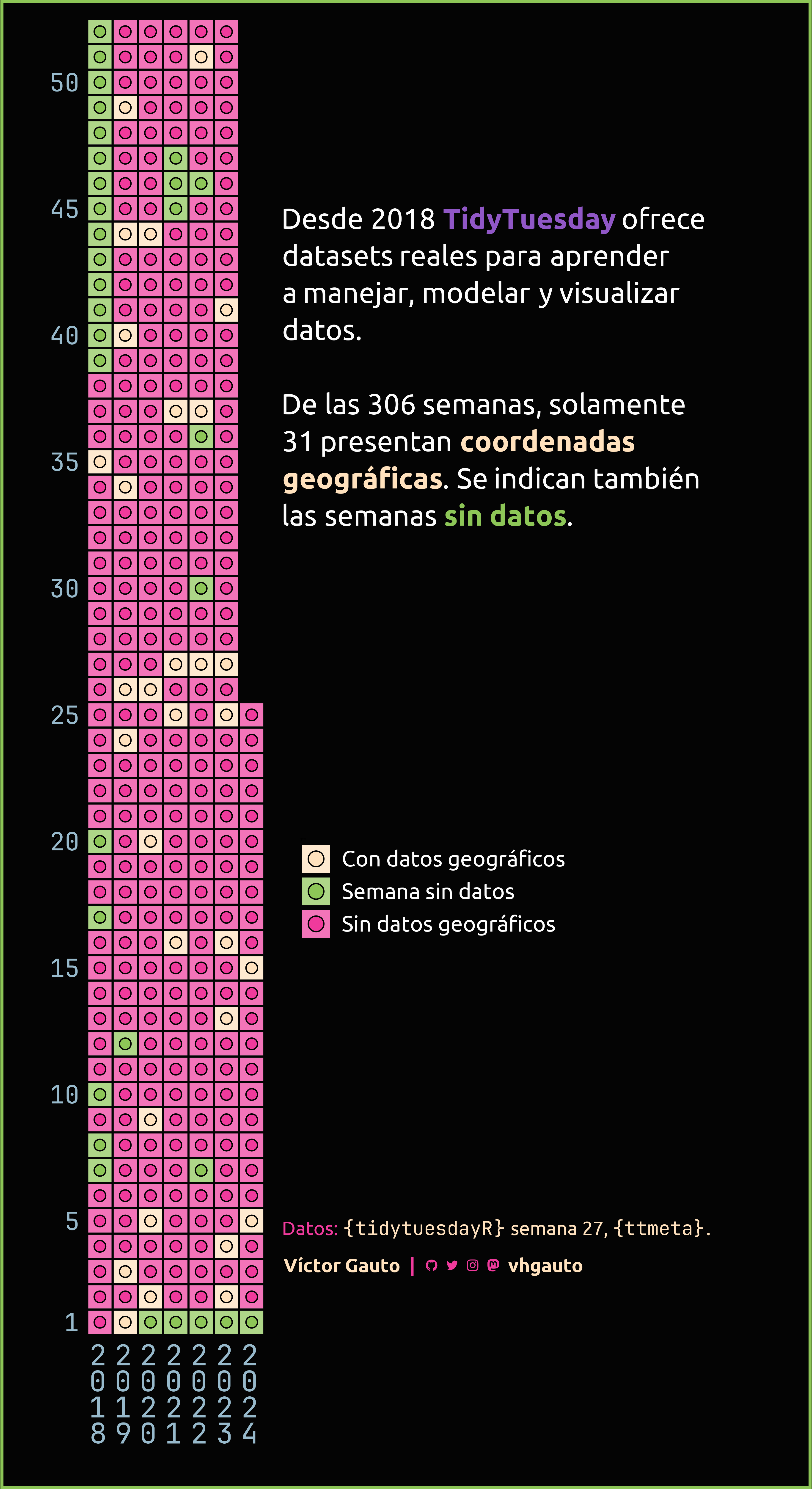
"Desde 2018 <b style='color:{pal[2]}'>TidyTuesday</b> ofrece",
"datasets reales para aprender",
"a manejar, modelar y visualizar",
"datos.<br>",
"De las {n_datasets} semanas, solamente",
"{n_geo} presentan <b style='color:{pal[3]}'>coordenadas",
"geográficas</b>. Se indican también",
"las semanas <b style='color:{pal[4]}'>sin datos</b>.",
.sep = "<br>"
)
# figura
g <- ggplot(e2, aes(year, week, color = geo, fill = geo)) +
geom_tile(
color = c1, linewidth = 1, show.legend = TRUE) +
geom_tile(
color = c1, fill = alpha(c2, .3), linewidth = 1,
show.legend = TRUE) +
geom_point(
size = 5, shape = 21, color = c1, stroke = 1, show.legend = TRUE) +
scale_x_continuous(
breaks = 2018:2024, limits = c(2017.5, 2024.5),
expand = c(0, 0), labels = eje_x_label) +
scale_y_continuous(
breaks = c(1, seq(5, 50, 5)), limits = c(.5, 52.5), expand = c(0, 0),
sec.axis = sec_axis(
breaks = c(45, 5),
labels = c(mi_subtitulo, mi_caption),
transform = ~ .
)) +
scale_color_manual(values = pal[3:5]) +
scale_fill_manual(values = pal[3:5]) +
guides(
color = guide_legend(position = "inside", override.aes = list(size = 7)),
fill = guide_legend(position = "inside", override.aes = list(size = 7))
) +
coord_fixed(clip = "off") +
theme_void(base_size = 4) +
theme(
plot.margin = margin(b = 15, r = 105, l = 50, t = 20),
plot.background = element_rect(fill = c1, color = pal[4], linewidth = 3),
plot.caption = element_markdown(
family = "ubuntu", size = 18, color = pal[5], margin = margin(r = -100)),
axis.text.x = element_markdown(
family = "jet", color = pal[1], size = 30, margin = margin(t = 10)),
axis.text.y = element_text(
family = "jet", color = pal[1], size = 26, margin = margin(r = 10),
hjust = 1),
axis.text.y.right = element_markdown(
family = "ubuntu", size = 30, hjust = 0, margin = margin(l = 20),
vjust = 1, lineheight = unit(1.3, "line"), color = c2),
legend.key.size = unit(1.2, "cm"),
legend.text = element_text(
color = c2, family = "ubuntu", size = 23, margin = margin(l = 10)),
legend.position.inside = c(1.2, .3),
legend.justification.inside = c(0, 0)
)
# guardo
ggsave(
plot = g,
filename = "2024/s27/viz.png",
width = 30,
height = 55,
units = "cm")
# abro
browseURL("2024/s27/viz.png")