Ocultar código
library(glue)
library(ggtext)
library(showtext)
library(tidyverse)
Sitio en construcción
Víctor Gauto
25 de marzo de 2025
Frecuencia de la palabra amazon
en los reportes anuales de Amazon.
Colores.
Fuentes: Ubuntu, JetBrains Mono y Bebas Neue.
font_add(
family = "ubuntu",
regular = "././fuente/Ubuntu-Regular.ttf",
bold = "././fuente/Ubuntu-Bold.ttf",
italic = "././fuente/Ubuntu-Italic.ttf"
)
font_add(
family = "jet",
regular = "././fuente/JetBrainsMonoNLNerdFontMono-Regular.ttf"
)
font_add(
family = "bebas",
regular = "././fuente/BebasNeue-Regular.ttf"
)
showtext_auto()
showtext_opts(dpi = 300)
fuente <- glue(
"Datos: <span style='color:{c1};'><span style='font-family:jet;'>",
"{{<b>tidytuesdayR</b>}}</span> semana 12, ",
"<b>Reporte anual de Amazon</b>.</span>"
)
autor <- glue("<span style='color:{c1};'>**Víctor Gauto**</span>")
icon_twitter <- glue("<span style='font-family:jet;'></span>")
icon_instagram <- glue("<span style='font-family:jet;'></span>")
icon_github <- glue("<span style='font-family:jet;'></span>")
icon_mastodon <- glue("<span style='font-family:jet;'>󰫑</span>")
icon_bsky <- glue("<span style='font-family:jet;'></span>")
usuario <- glue("<span style='color:{c1};'>**vhgauto**</span>")
sep <- glue("**|**")
mi_caption <- glue(
"{fuente}<br>{autor} {sep} {icon_github} {icon_twitter} {icon_instagram} ",
"{icon_mastodon} {icon_bsky} {usuario}"
)
Me interesa la cantidad de veces que aparece la palabra amazon
en cada reporte anual.
Logo de Amazon, título y descripción.
link <- "https://upload.wikimedia.org/wikipedia/commons/thumb/0/06/Amazon_2024.svg/960px-Amazon_2024.svg.png"
logo <- glue("<img src='{link}' width=110 />")
mi_titulo <- glue(
"{logo} hablando de {logo}"
)
mi_subtitulo <- glue(
"Cantidad de veces que aparece la palabra
<b style='color: {c1}'>amazon</b><br> en los reportes anuales de
<b style='color: {c1}'>amazon</b>."
)
Figura.
g <- ggplot(d, aes(year, n)) +
geom_line(
color = c1, linewidth = 5, arrow = arrow(), lineend = "round"
) +
geom_point(data = slice(d, 1:(nrow(d)-1)), color = c4, size = 2) +
annotate(
geom = "richtext", x = I(1), y = I(.25), label = mi_subtitulo, fill = c4,
label.color = NA, size = 7, family = "ubuntu", hjust = 1
) +
scale_x_continuous(limits = c(2002.5, 2023)) +
scale_y_continuous(limits = c(-17, 220)) +
coord_cartesian(expand = FALSE, clip = "off") +
labs(title = mi_titulo, caption = mi_caption) +
theme_void() +
theme(
text = element_text(color = c2),
aspect.ratio = 1,
plot.margin = margin(25, 5, 15, 5),
plot.background = element_rect(fill = c4, color = NA),
plot.title.position = "plot",
plot.title = element_markdown(
family = "ubuntu", color = c2, size = 50, margin = margin(b = 25),
hjust = .5
),
plot.caption = element_markdown(
family = "ubuntu", size = 15, color = c2, margin = margin(t = 25),
lineheight = 1.1
),
panel.grid.major = element_line(linewidth = .2, color = c3, linetype = 1),
axis.text = element_text(
family = "bebas", color = c3, face = "bold", size = 70
),
axis.text.x = element_text(hjust = -0.03, margin = margin(t = -53)),
axis.text.y = element_text(
vjust = -.1, margin = margin(r = -90), hjust = 1
)
)
Guardo.
---
format:
html:
code-fold: show
code-summary: "Ocultar código"
code-line-numbers: false
code-annotations: false
code-link: true
code-tools:
source: true
toggle: true
caption: "Código"
code-overflow: scroll
page-layout: full
editor_options:
chunk_output_type: console
categories: ["geom_line", "geom_point"]
execute:
eval: false
echo: true
warning: false
title: "Semana 12"
date: 2025-03-25
author: Víctor Gauto
---
Frecuencia de la palabra `amazon` en los reportes anuales de <b>Amazon</b>.

## Paquetes
```{r}
library(glue)
library(ggtext)
library(showtext)
library(tidyverse)
```
## Estilos
Colores.
```{r}
c1 <- "#FF6200"
c2 <- "#101722"
c3 <- "grey80"
c4 <- "grey90"
```
Fuentes: Ubuntu, JetBrains Mono y Bebas Neue.
```{r}
font_add(
family = "ubuntu",
regular = "././fuente/Ubuntu-Regular.ttf",
bold = "././fuente/Ubuntu-Bold.ttf",
italic = "././fuente/Ubuntu-Italic.ttf"
)
font_add(
family = "jet",
regular = "././fuente/JetBrainsMonoNLNerdFontMono-Regular.ttf"
)
font_add(
family = "bebas",
regular = "././fuente/BebasNeue-Regular.ttf"
)
showtext_auto()
showtext_opts(dpi = 300)
```
## Epígrafe
```{r}
fuente <- glue(
"Datos: <span style='color:{c1};'><span style='font-family:jet;'>",
"{{<b>tidytuesdayR</b>}}</span> semana 12, ",
"<b>Reporte anual de Amazon</b>.</span>"
)
autor <- glue("<span style='color:{c1};'>**Víctor Gauto**</span>")
icon_twitter <- glue("<span style='font-family:jet;'></span>")
icon_instagram <- glue("<span style='font-family:jet;'></span>")
icon_github <- glue("<span style='font-family:jet;'></span>")
icon_mastodon <- glue("<span style='font-family:jet;'>󰫑</span>")
icon_bsky <- glue("<span style='font-family:jet;'></span>")
usuario <- glue("<span style='color:{c1};'>**vhgauto**</span>")
sep <- glue("**|**")
mi_caption <- glue(
"{fuente}<br>{autor} {sep} {icon_github} {icon_twitter} {icon_instagram} ",
"{icon_mastodon} {icon_bsky} {usuario}"
)
```
## Datos
```{r}
tuesdata <- tidytuesdayR::tt_load(2025, 12)
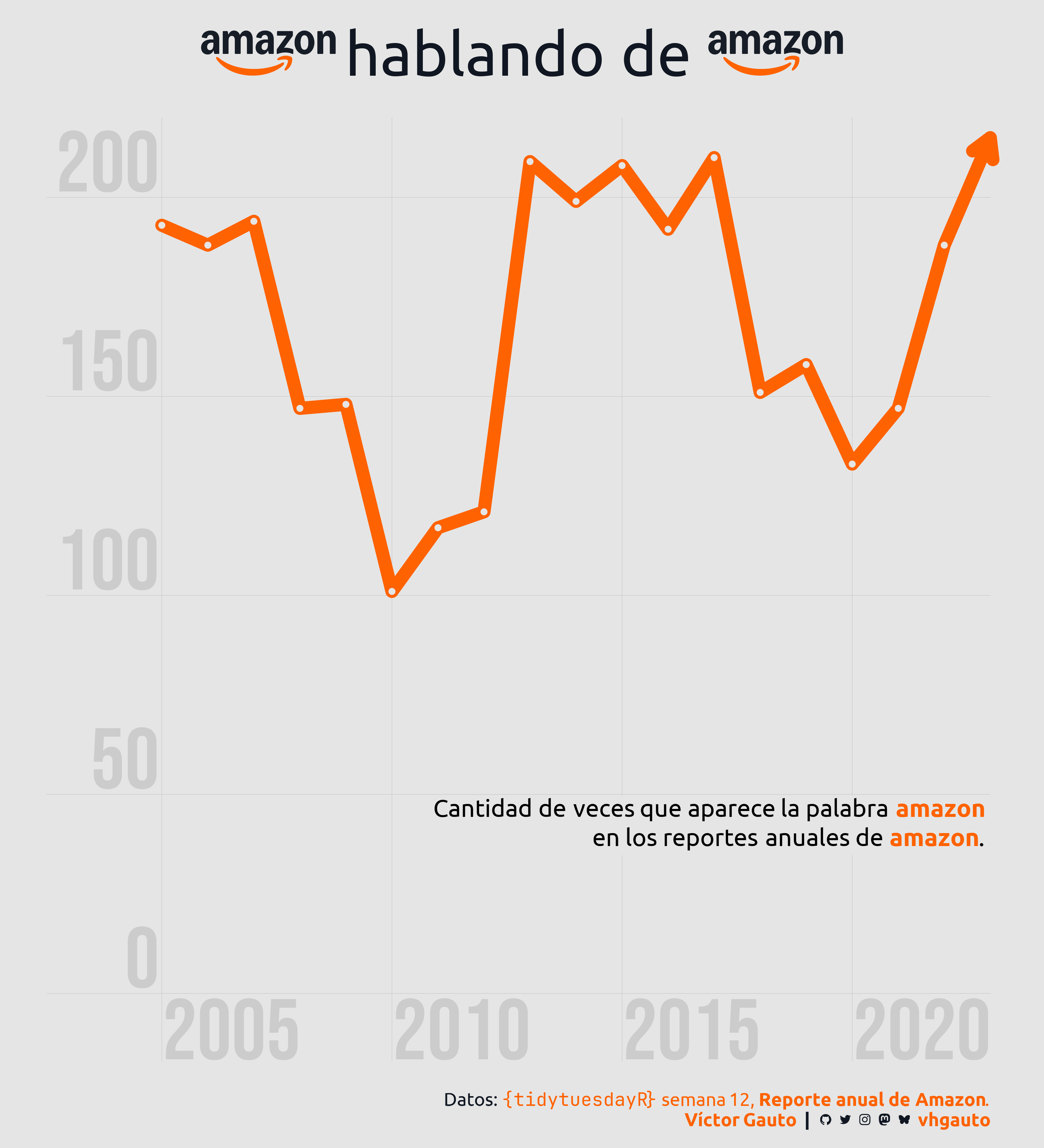
palabras <- tuesdata$report_words_clean
```
## Procesamiento
Me interesa la cantidad de veces que aparece la palabra `amazon` en cada reporte anual.
```{r}
d <- palabras |>
filter(str_detect(word, "amazon")) |>
count(year)
```
## Figura
Logo de Amazon, título y descripción.
```{r}
link <- "https://upload.wikimedia.org/wikipedia/commons/thumb/0/06/Amazon_2024.svg/960px-Amazon_2024.svg.png"
logo <- glue("<img src='{link}' width=110 />")
mi_titulo <- glue(
"{logo} hablando de {logo}"
)
mi_subtitulo <- glue(
"Cantidad de veces que aparece la palabra
<b style='color: {c1}'>amazon</b><br> en los reportes anuales de
<b style='color: {c1}'>amazon</b>."
)
```
Figura.
```{r}
g <- ggplot(d, aes(year, n)) +
geom_line(
color = c1, linewidth = 5, arrow = arrow(), lineend = "round"
) +
geom_point(data = slice(d, 1:(nrow(d)-1)), color = c4, size = 2) +
annotate(
geom = "richtext", x = I(1), y = I(.25), label = mi_subtitulo, fill = c4,
label.color = NA, size = 7, family = "ubuntu", hjust = 1
) +
scale_x_continuous(limits = c(2002.5, 2023)) +
scale_y_continuous(limits = c(-17, 220)) +
coord_cartesian(expand = FALSE, clip = "off") +
labs(title = mi_titulo, caption = mi_caption) +
theme_void() +
theme(
text = element_text(color = c2),
aspect.ratio = 1,
plot.margin = margin(25, 5, 15, 5),
plot.background = element_rect(fill = c4, color = NA),
plot.title.position = "plot",
plot.title = element_markdown(
family = "ubuntu", color = c2, size = 50, margin = margin(b = 25),
hjust = .5
),
plot.caption = element_markdown(
family = "ubuntu", size = 15, color = c2, margin = margin(t = 25),
lineheight = 1.1
),
panel.grid.major = element_line(linewidth = .2, color = c3, linetype = 1),
axis.text = element_text(
family = "bebas", color = c3, face = "bold", size = 70
),
axis.text.x = element_text(hjust = -0.03, margin = margin(t = -53)),
axis.text.y = element_text(
vjust = -.1, margin = margin(r = -90), hjust = 1
)
)
```
Guardo.
```{r}
ggsave(
plot = g,
filename = "tidytuesday/2025/semana_12.png",
width = 30,
height = 33,
units = "cm"
)
```