Semana 47

Figura semana 47

Eventos R-Ladies de Argentina.

Script

# paquetes ----------------------------------------------------------------

library(tidyverse)
library(glue)
library(sf)
library(ggtext)
library(showtext)

# fuente ------------------------------------------------------------------

# colores
c1 <- "#E8631C"
c2 <- "#E3D885"
c3 <- "white"
c4 <- "#6874AD"
c5 <- "#0D2D4C"
c6 <- "#20222A"

# texto gral
font_add_google(name = "Ubuntu", family = "ubuntu")
# números, fechas, ranking
font_add_google(name = "Victor Mono", family = "victor", db_cache = FALSE)
# título
font_add_google(name = "Bebas Neue", family = "bebas")

# íconos
font_add("fa-brands", "icon/Font Awesome 6 Brands-Regular-400.otf")

showtext_auto()
showtext_opts(dpi = 300)

# caption
fuente <- glue(
  "Datos: <span style='color:{c3};'><span style='font-family:mono;'>",
  "{{<b>tidytuesdayR</b>}}</span> semana 47. ",
  "R-Ladies Chapters: Making talks work for diverse audiences, ",
  "**Federica Gazzelloni**</span>")
autor <- glue("<span style='color:{c3};'>**Víctor Gauto**</span>")
icon_twitter <- glue("<span style='font-family:fa-brands;'>&#xf099;</span>")
icon_github <- glue("<span style='font-family:fa-brands;'>&#xf09b;</span>")
icon_mastodon <- glue("<span style='font-family:fa-brands;'>&#xf4f6;</span>")
usuario <- glue("<span style='color:{c3};'>**vhgauto**</span>")
sep <- glue("**|**")

mi_caption <- glue(
  "{fuente}<br>{autor} {sep} {icon_github} {icon_twitter} {icon_mastodon} 
  {usuario}")

# datos -------------------------------------------------------------------

browseURL("https://github.com/rfordatascience/tidytuesday/blob/master/data/2023/2023-11-21/readme.md")

rladies <- readr::read_csv('https://raw.githubusercontent.com/rfordatascience/tidytuesday/master/data/2023/2023-11-21/rladies_chapters.csv')

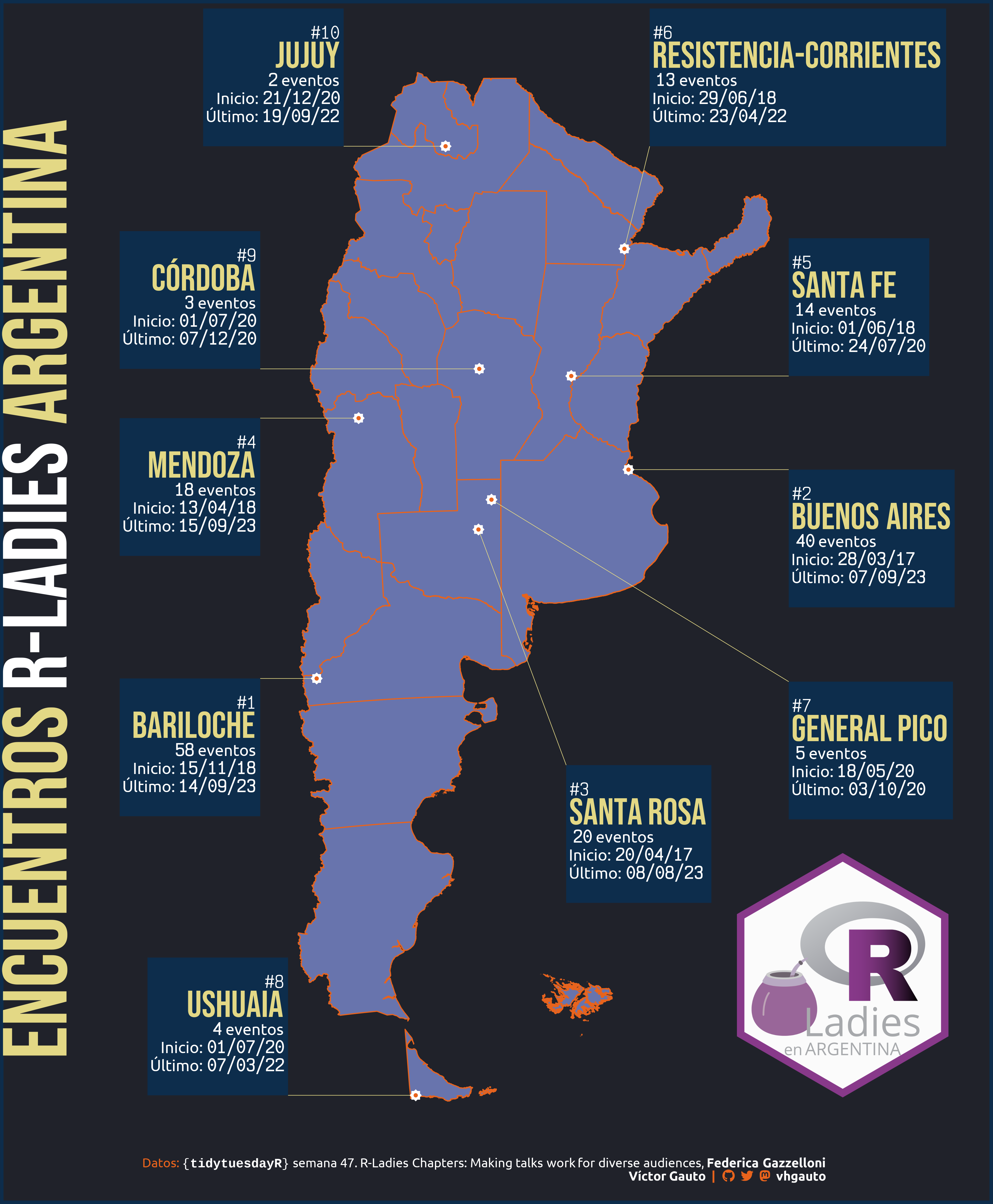
# me interesa hacer un mapa con los encuentros de Argentina, en qué ciudades, 
# la cantidad, fecha inicial y final

# provincias de Argentina, POSGAR
pcias <- st_read("2023/semana_47/pcias_continental.gpkg")

# ciudades de Argentina donde se realizaron eventos, obtenido de:
browseURL("https://rladies.org/")

ciudades <- c(
  "bariloche", "buenos-aires", "cordoba", "general-pico", "jujuy", "mendoza",
  "resistencia-corrientes", "santa-fe", "santa-rosa", "ushuaia")

# nombres de las ciudades
ciudades_nombres <- c(
  "Bariloche", "Buenos Aires", "Santa Rosa", "Mendoza", "Santa Fe", 
  "Resistencia-Corrientes", "General Pico", "Ushuaia", "Córdoba", "Jujuy")

# coordenadas de las ciudades
ciudad_lon <- c(
  -71.300000, -58.381944, -64.290556, -68.833333, -60.700000, -58.861760,
  -63.757766, -68.304444, -64.183333, -65.299444)
ciudad_lat <- c(
  -41.150000, -34.599722, -36.620278, -32.883333, -31.633333, -27.468502,
  -35.658688, -54.807222, -31.416667, -24.185556)

# creo un sf con las coordenadas de las ciudades, POSGAR
ciudades_pts <- tibble(
  ciudad = ciudades_nombres) |> 
  mutate(x = ciudad_lon, y = ciudad_lat) |> 
  st_as_sf(coords = c("x", "y")) |> 
  st_set_crs(value = 4326) |> 
  st_transform(crs = st_crs(pcias))

# coordenadas de las ciudades, tibble
ciudades_pts_tbl <- ciudades_pts |> 
  st_coordinates() |> 
  as_tibble()
  
# cantidad de eventos, fecha del primer/útlimo evento, nombre de la ciudad, 
# ranking
ciudades_tbl <- rladies |> 
  mutate(chapter = str_remove(chapter, "rladies-")) |> 
  filter(chapter %in% ciudades) |> 
  reframe(
    n = n(),
    fecha_i = min(date),
    fecha_f = max(date),
    .by = chapter) |> 
  arrange(desc(n)) |> 
  mutate(nombre = ciudades_nombres) |> 
  mutate(puesto = row_number())

# longitud de las etiquetas
der <- 5500000
izq <- 3600000

# etiquetas por ciudad
d <- ciudades_tbl |> 
  mutate(fecha_i = format(fecha_i, "%d/%m/%y")) |> 
  mutate(fecha_f = format(fecha_f, "%d/%m/%y")) |> 
  mutate(label = glue(
    "<br><span style='font-family:victor;font-size:15pt;color:{c3}'>#{puesto}</span>",
    "<span style='font-family:bebas;font-size:35pt;color:{c2}'>{nombre}</span>",
    "<span style='font-size:15pt;color:{c3}'> <b style='font-family:victor'>{n}</b> eventos",
    "Inicio: <b style='font-family:victor'>{fecha_i}</b>",
    "Último: <b style='font-family:victor'>{fecha_f}</b>",
    "</span>",
    .sep = "<br>")) |> 
  mutate(
    x = ciudades_pts_tbl$X,
    y = ciudades_pts_tbl$Y,
    xend = c(
      izq, der, 4700000, izq, der, 5000000, der, 3700000, izq, 3900000),
    yend = c(
      5411386, 6162069, 5100000, 6347028, 6498473, 7324204, 5400000, 3913285, 
      6524189, 7324204),
    hjust = c(1, 0, 0, 1, 0, 0, 0, 1, 1, 1),
    vjust = c(1, 1, 1, 1, 0, 0, 1, 0, 0, 0))

# figura ------------------------------------------------------------------

# logo de R-Ladies Argentina
logo <- "2023/semana_47/logo.png"
logo_label <- glue("<img src='{logo}' width='200'>")

# título
tit_tbl <- tibble(
  x = 2800000,
  y = 5740431,
  label = glue("Encuentros <span style='color:{c3}'>R-Ladies</span> Argentina"))

# figura
g <- ggplot() +
  # provincias de Argentina
  geom_sf(data = pcias, fill = c4, color = c1, linewidth = .5) +
  # líneas entre ciudad y etiqueta
  geom_segment(
    data = d, aes(x, y, xend = xend, yend = yend), color = c2,
    linewidth = .25, linetype = 1) +
  # puntos de ciudades
  geom_sf(data = ciudades_pts, color = c3, size = 3.5, shape = 15) +
  geom_sf(data = ciudades_pts, color = c3, size = 5, shape = 18) +
  geom_sf(data = ciudades_pts, color = c1, size = 2, shape = 20) +
  # etiquetas
  geom_richtext(
    data = d, aes(xend, yend, label = label, hjust = hjust, vjust = vjust), 
    fill = c5, label.color = NA, label.r = unit(0, "mm"), size = 4,
    family = "ubuntu", color = c3, lineheight = unit(1.5, "mm")) +
  # título
  geom_richtext(
    data = tit_tbl, aes(x, y, label = label), angle = 90, color = c2,
    size = 30, family = "bebas", fill = NA, label.color = NA) +
  # logo R-Ladies Argentina
  annotate(
    geom = "richtext", x = 5300000, y = 3891909, hjust = 0, vjust = 0,
    label = logo_label, fill = NA, label.color = NA, label.r = unit(0, "mm")) +
  coord_sf(clip = "off") +
  labs(caption = mi_caption) +
  theme_void() +
  theme(
    plot.background = element_rect(fill = c6, color = c5, linewidth = 3),
    plot.margin = margin(20, 157.5, 20, 0),
    plot.caption.position = "plot",
    plot.caption = element_markdown(
      family = "ubuntu", size = 12, color = c1))

# guardo
ggsave(
  plot = g,
  filename = "2023/semana_47/viz.png",
  width = 33,
  height = 40,
  units = "cm")

# abro
browseURL("2023/semana_47/viz.png")

Figura