# paquetes ----------------------------------------------------------------
library(glue)
library(ggtext)
library(showtext)
library(ggthemes)
library(patchwork)
library(tidyverse)
# fuente ------------------------------------------------------------------
# colores
pal <- c("#F28AAA", "#A1C2ED", "#9CC184", "#F9D14A", "#DF9ED4")
c1 <- "#EAF3FF"
c2 <- "white"
c3 <- "grey10"
c4 <- "grey90"
# fuente: Ubuntu
font_add(
family = "ubuntu",
regular = "fuente/Ubuntu-Regular.ttf",
bold = "fuente/Ubuntu-Bold.ttf",
italic = "fuente/Ubuntu-Italic.ttf"
)
# monoespacio & íconos
font_add(
family = "jet",
regular = "fuente/JetBrainsMonoNLNerdFontMono-Regular.ttf"
)
font_add_google(
name = "Ultra",
family = "ultra"
)
showtext_auto()
showtext_opts(dpi = 300)
# caption
fuente <- glue(
"Datos: <span style='color:{pal[4]};'><span style='font-family:jet;'>",
"{{<b>tidytuesdayR</b>}}</span> semana {35}, ",
"Power Rangers Dataset.</span>"
)
autor <- glue("<span style='color:{pal[4]};'>**Víctor Gauto**</span>")
icon_twitter <- glue("<span style='font-family:jet;'></span>")
icon_instagram <- glue("<span style='font-family:jet;'></span>")
icon_github <- glue("<span style='font-family:jet;'></span>")
icon_mastodon <- glue("<span style='font-family:jet;'>󰫑</span>")
icon_imdb <- glue(
"<span style='font-family:jet; font-size:40px'></span>")
usuario <- glue("<span style='color:{pal[4]};'>**vhgauto**</span>")
sep <- glue("**|**")
mi_caption <- glue(
"{fuente}<br>{autor} {sep} {icon_github} {icon_twitter} ",
"{icon_instagram} {icon_mastodon} {usuario}"
)
url_pr <- "https://upload.wikimedia.org/wikipedia/en/b/bd/Power_Rangers_Logo.webp"
# datos -------------------------------------------------------------------
tuesdata <- tidytuesdayR::tt_load(2024, 35)
episodes <- tuesdata$power_rangers_episodes
# me interesa la popularidad y el puntaje de los episodios al inicio y en la
# actualidad de la serie
# agrego el año de inicio a la temporada
d <- episodes |>
mutate(season_title = str_replace(season_title, "Season ", "T")) |>
mutate(año_i = year(min(air_date)), .by = season_title) |>
mutate(
año_i = glue(
"<span style='font-family: jet; font-size: 15px; color: {pal[1]}'>",
"{año_i}</span>"
)
) |>
mutate(season_title = glue("{season_title}<br>{año_i}")) |>
mutate(season_title = fct_reorder(season_title, air_date))
# cantidad de temporadas
n_season <- length(unique(d$season_title))
# figura ------------------------------------------------------------------
# título de los ejes
eje_horizontal <- glue("Votos<br>{icon_imdb}")
eje_vertical <- glue("Puntaje<br>{icon_imdb}")
# función que genera una figura para las primeras/últimas temporadas
f_gg <- function(tbl, subtitulo) {
g <- ggplot(tbl, aes(total_votes, IMDB_rating, fill = season_title)) +
# todas las temporadas
geom_point(
data = select(d, -season_title), aes(total_votes, IMDB_rating),
inherit.aes = FALSE, alpha = .1, size = .6, show.legend = FALSE,
color = c2, shape = 20
) +
# temporadas de interés, a destacar
geom_point(
alpha = .9, size = 2, show.legend = FALSE, shape = 21
) +
facet_wrap(vars(season_title), ncol = 5, scales = "free") +
scale_x_log10(
limits = c(10, 1000), expand = c(0, 0), breaks = c(10, 100, 1000)
) +
scale_y_continuous(limits = c(4, 10), expand = c(0, 0), breaks = 4:10) +
scale_fill_manual(
values = rep(pal, length.out = n_season)
) +
labs(x = eje_horizontal, y = eje_vertical, subtitle = subtitulo) +
coord_cartesian(clip = "off") +
theme_linedraw() +
theme(
aspect.ratio = 1,
plot.margin = margin(b = -20),
plot.background = element_blank(),
plot.subtitle = element_markdown(
size = 16, family = "ubuntu", color = c1, margin = margin(b = 5, t = 20)
),
panel.background = element_blank(),
panel.grid = element_blank(),
panel.spacing.x = unit(1.3, "line"),
axis.ticks = element_blank(),
axis.title.x = element_markdown(
family = "ubuntu", hjust = .1, margin = margin(t = 10), color = c2
),
axis.title.y = element_markdown(
family = "ubuntu", angle = 0, vjust = .5, margin = margin(r = 10),
color = c2
),
axis.text = element_text(family = "jet", color = c2),
axis.text.y = element_text(vjust = 0),
strip.text = element_markdown(
hjust = 0, family = "ubuntu", color = pal[2], size = 13, face = "bold"
),
strip.background = element_blank()
)
return(g)
}
# número de las primeras/últimas temporadas
n_head <- unique(as.numeric(d$season_title))[1:5]
n_tail <- unique(as.numeric(d$season_title))[(n_season-4):n_season]
# filtro a partir del número de las primeras/últimas temporadas
d_head <- d |>
filter(as.numeric(season_title) %in% n_head)
d_tail <- d |>
filter(as.numeric(season_title) %in% n_tail)
# subtítulo de cada figura
pr <- glue(
"<span style='font-family: ultra; color: {pal[4]};'>POWER RANGERS</span>"
)
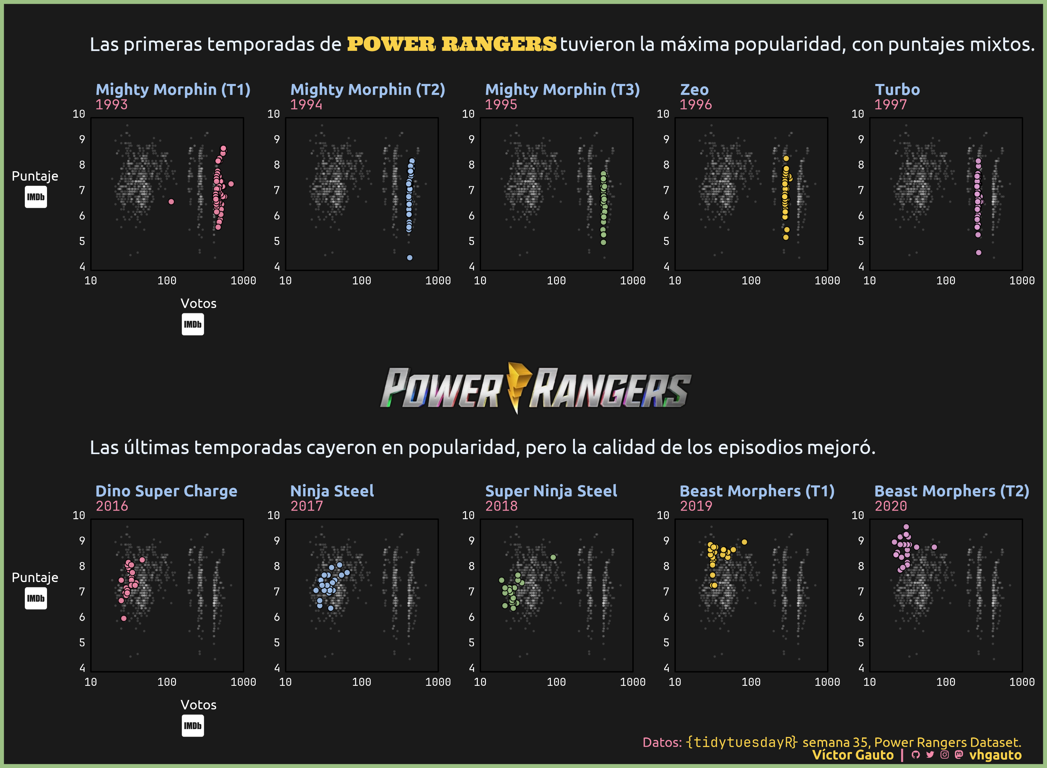
sub_head <- glue(
"Las primeras temporadas de {pr} tuvieron la máxima popularidad, ",
"con puntajes mixtos."
)
sub_tail <- glue(
"Las últimas temporadas cayeron en popularidad, pero la calidad de los ",
"episodios mejoró."
)
# logo de los Power Rangers
g_pr <- ggplot() +
ggpath::geom_from_path(
data = tibble(x = 0, y = 0, path = url_pr),
aes(x, y, path = path)) +
coord_cartesian(xlim = c(-.02, .02212), clip = "off") +
theme_void()
# composición final de la figura
g <- f_gg(d_head, sub_head) / g_pr / f_gg(d_tail, sub_tail) +
plot_layout(heights = c(.43, .13, .43)) +
plot_annotation(
caption = mi_caption,
theme = theme(
plot.margin = margin(r = 20, l = 10, t = 10, b = 5),
plot.background = element_rect(fill = c3, color = pal[3], linewidth = 3),
plot.caption = element_markdown(
family = "ubuntu", size = 11, color = pal[1], margin = margin(t = -20)
)
)
)
# guardo
ggsave(
plot = g,
filename = "2024/s35/viz.png",
width = 30,
height = 22,
units = "cm")
# abro
browseURL(glue("{getwd()}/2024/s35/viz.png"))