Semana 40

Figura semana 40

Oportunidades de subvención del Gobierno de EEUU.

Script

# paquetes ----------------------------------------------------------------

library(tidyverse)
library(glue)
library(ggrepel)
library(ggtext)
library(showtext)

# fuente ------------------------------------------------------------------

# colores, Isfahan
c1 <- "#E3C28B"
c2 <- "#AE8448"
c3 <- "#175F5D"
c4 <- "#4E3810"
c5 <- "#054544"

# agencias, texto gral
font_add_google(name = "Ubuntu", family = "ubuntu")
# ejes vertical  horizontal
font_add_google(name = "Victor Mono", family = "victor", db_cache = FALSE)
# título
font_add_google(name = "Lora", family = "lora")

# íconos
font_add("fa-brands", "icon/Font Awesome 6 Brands-Regular-400.otf")
font_add("fa-solids", "icon/Font Awesome 6 Free-Solid-900.otf")

showtext_auto()
showtext_opts(dpi = 300)

# caption
fuente <- glue("Datos: <span style='color:{c3};'><span style='font-family:victor;'>{{<b>tidytuesdayR</b>}}</span> semana 40. US Government Grant Opportunities, *grants.gov*</span>")
autor <- glue("Autor: <span style='color:{c3};'>**Víctor Gauto**</span>")
icon_twitter <- glue("<span style='font-family:fa-brands;'>&#xf099;</span>")
icon_github <- glue("<span style='font-family:fa-brands;'>&#xf09b;</span>")
usuario <- glue("<span style='color:{c3};'>**vhgauto**</span>")
sep <- glue("**|**")

mi_caption <- glue("{fuente}<br>{autor} {sep} {icon_github} {icon_twitter} {usuario}")

# datos -------------------------------------------------------------------

browseURL("https://github.com/rfordatascience/tidytuesday/blob/master/data/2023/2023-10-03/readme.md")

grants <- readr::read_csv('https://raw.githubusercontent.com/rfordatascience/tidytuesday/master/data/2023/2023-10-03/grants.csv')

# me interesa la relación entre cantidad de oportunidades de las agencias, y 
# la cantidad de dinero estimada, por oprtunidad

# selecciono las 100 agencias con mayor presencia
agencia <- grants |> 
  drop_na(estimated_funding) |> 
  count(agency_name, sort = TRUE) |> 
  slice(1:100) |> 
  pull(agency_name)

# calculo el cociente entre dinero estimado y número de presentaciones
# obtengo la distancia de cada punto respecto del origen
d <- grants |> 
  filter(agency_name %in% agencia) |> 
  drop_na(estimated_funding) |> 
  summarise(
    cantidad = n(),
    tot = sum(estimated_funding),
    .by = agency_name) |> 
  mutate(ratio = tot/cantidad) |> 
  mutate(distancia = sqrt(tot^2 + ratio^2))

# puntos extremos
e <- d |> 
  filter(
    cantidad == max(d$cantidad) | 
      cantidad == min(d$cantidad) |
      ratio == max(d$ratio) | ratio == min(d$ratio) |
      distancia == max(d$distancia) | distancia == min(d$distancia)) |> 
  mutate(label = str_wrap(agency_name, width = 20)) |> 
  mutate(hjust = c())

# selecciono dos casos extremos, de muchas presentaciones con poca plata,
# y pocas presentaciones con mucha plata
nps <- e |> 
  filter(agency_name == "National Park Service")

nps_cantidad <- nps$cantidad |> 
  gt::vec_fmt_number(sep_mark = ".", decimals = 0, dec_mark = ",")

nps_ratio <- nps$ratio |> 
  gt::vec_fmt_number(sep_mark = ".", decimals = 0, dec_mark = ",")

afo <- e |> 
  filter(agency_name == "Air Force Office of Scientific Research")

afo_cantidad <- afo$cantidad |> 
  gt::vec_fmt_number(sep_mark = ".", decimals = 0, dec_mark = ",")

afo_ratio <- afo$ratio |> 
  gt::vec_fmt_number(sep_mark = ".", decimals = 0, dec_mark = ",")

# figura ------------------------------------------------------------------

# tpitulo & subtítulo
mi_title <- "Subvenciones by *grants.gov*"
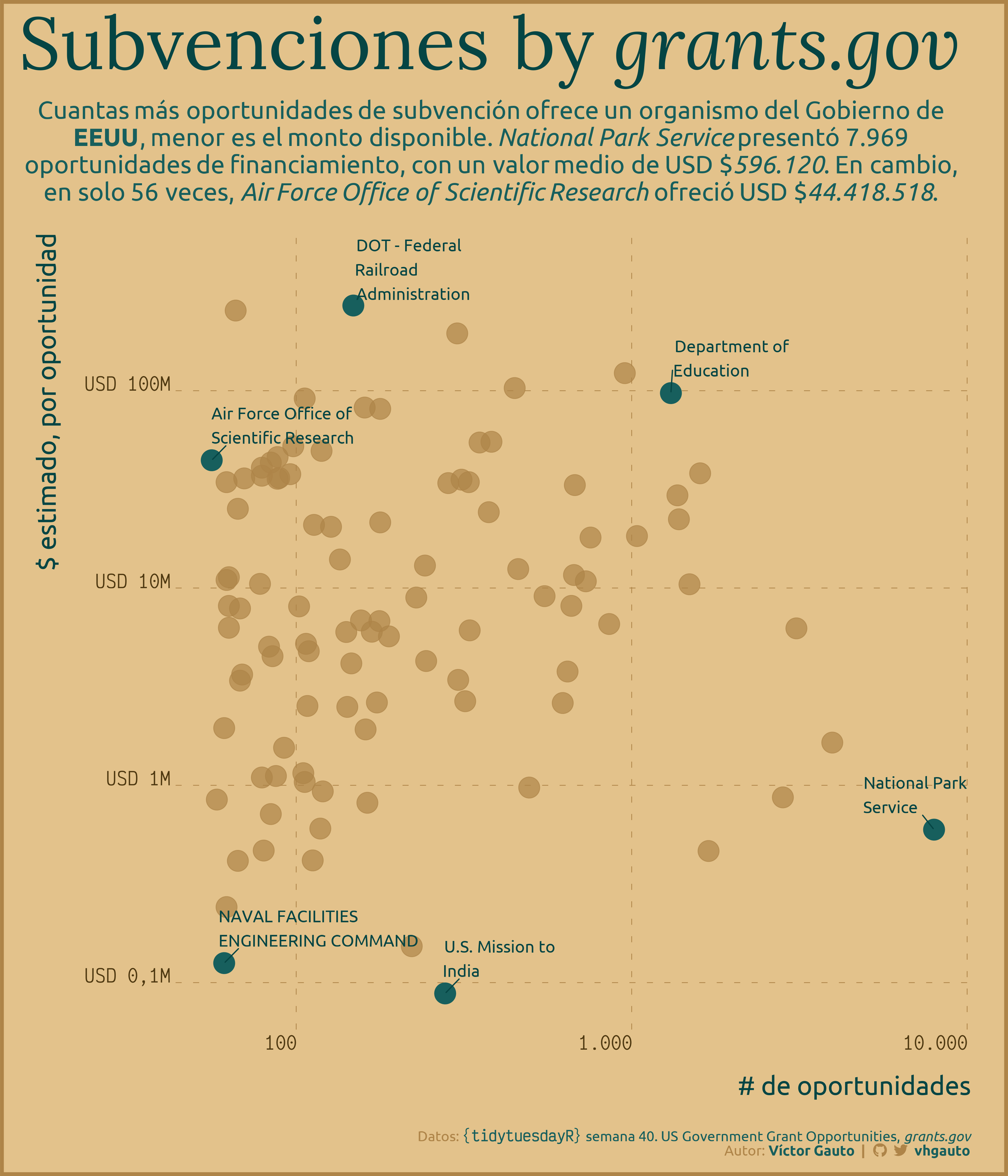
mi_sub <- glue(
  "Cuantas más oportunidades de subvención ofrece un organismo del 
  Gobierno de<br>**EEUU**, menor es el monto disponible. *{nps$agency_name}* 
  presentó {nps_cantidad}<br>oportunidades de financiamiento,
  con un valor medio de USD $*{nps_ratio}*. En cambio,<br>en solo {afo_cantidad}
  veces, *{afo$agency_name}* ofreció USD $*{afo_ratio}*.")

# figura
g <- d |> 
  mutate(tipo = agency_name %in% e$agency_name) |> 
  ggplot(aes(cantidad, ratio, color = tipo, alpha = tipo)) +
  geom_point(size = 8, show.legend = FALSE) +
  geom_text_repel(
    data = e, aes(cantidad, ratio, label = label), inherit.aes = FALSE,
    hjust = 0, color = c5, seed = 2024, nudge_y = .175, family = "ubuntu",
    size = 5) +
  scale_x_log10(
    labels = scales::label_number(decimal.mark = ",", big.mark = ".")) +
  scale_y_log10(
    breaks = c(1e5, 1e6, 10e6, 100e6),
    labels = glue("USD {c('0,1', '1', '10', '100')}M")) +
  scale_color_manual(values = c(c2, c3)) +
  scale_alpha_manual(values = c(.7, 1)) +
  coord_cartesian(clip = "off") +
  labs(
    title = mi_title,
    subtitle = mi_sub,
    x = "# de oportunidades",
    y = "$ estimado, por oportunidad",
    caption = mi_caption) +
  theme_minimal() +
  theme(
    aspect.ratio = 1,
    plot.margin = margin(15, 32, 15, 12),
    plot.background = element_rect(fill = c1, color = c2, linewidth = 3),
    plot.title = element_markdown(
      size = 62, color = c5, family = "lora", hjust = .5),
    plot.title.position = "plot",
    plot.subtitle = element_markdown(
      family = "ubuntu", size = 21, color = c3, margin = margin(5, 0, 25, 0),
      lineheight = unit(1.1, "line"), hjust = .5),
    plot.caption = element_markdown(color = c2, family = "ubuntu", size = 12),
    axis.text = element_text(family = "victor", color = c4, size = 15),
    axis.text.x = element_text(hjust = 1),
    axis.text.y = element_text(vjust = 0),
    axis.title.x = element_text(
      family = "ubuntu", size = 22, hjust = 1, color = c5, 
      margin = margin(20, 0, 20, 0)),
    axis.title.y = element_text(
      family = "ubuntu", size = 22, hjust = 1, color = c5, 
      margin = margin(0, 20, 0, 20)),
    panel.grid.minor = element_blank(),
    panel.grid.major = element_line(
      color = c2, linewidth = .3, linetype = "8f")
  )

# guardo
ggsave(
  plot = g,
  filename = "2023/semana_40/viz.png",
  width = 30,
  height = 35,
  units = "cm")

# abro
browseURL("2023/semana_40/viz.png")

Figura