Ocultar código
library(glue)
library(ggtext)
library(showtext)
library(terra)
library(tidyterra)
library(marquee)
library(tidyverse)Eventos sísmicos en el Monte Vesubio.
library(glue)
library(ggtext)
library(showtext)
library(terra)
library(tidyterra)
library(marquee)
library(tidyverse)Colores.
c1 <- "violetred"
c2 <- "#FEFED7"
c3 <- "#081C57"
Fuentes: Ubuntu y JetBrains Mono.
font_add(
  family = "ubuntu",
  regular = "././fuente/Ubuntu-Regular.ttf",
  bold = "././fuente/Ubuntu-Bold.ttf",
  italic = "././fuente/Ubuntu-Italic.ttf"
)

font_add(
  family = "jet",
  regular = "././fuente/JetBrainsMonoNLNerdFontMono-Regular.ttf"
)

showtext_auto()
showtext_opts(dpi = 300)fuente <- glue(
"Datos: <span style='color:{c1};'><span style='font-family:jet;'>",
"{{<b>tidytuesdayR</b>}}</span> semana 19, ",
"<b>Italian Istituto Nazionale di Geofisica e Vulcanologia</b>.</span>"
)
autor <- glue("<span style='color:{c1};'>**Víctor Gauto**</span>")
icon_twitter <- glue("<span style='font-family:jet;'></span>")
icon_instagram <- glue("<span style='font-family:jet;'></span>")
icon_github <- glue("<span style='font-family:jet;'></span>")
icon_mastodon <- glue("<span style='font-family:jet;'>󰫑</span>")
icon_bsky <- glue("<span style='font-family:jet;'></span>")
usuario <- glue("<span style='color:{c1};'>**vhgauto**</span>")
sep <- glue("**|**")
mi_caption <- glue(
"{fuente}<br>{autor} {sep} {icon_github} {icon_twitter} {icon_instagram} ",
"{icon_mastodon} {icon_bsky} {usuario}"
)tuesdata <- tidytuesdayR::tt_load(2025, 19)
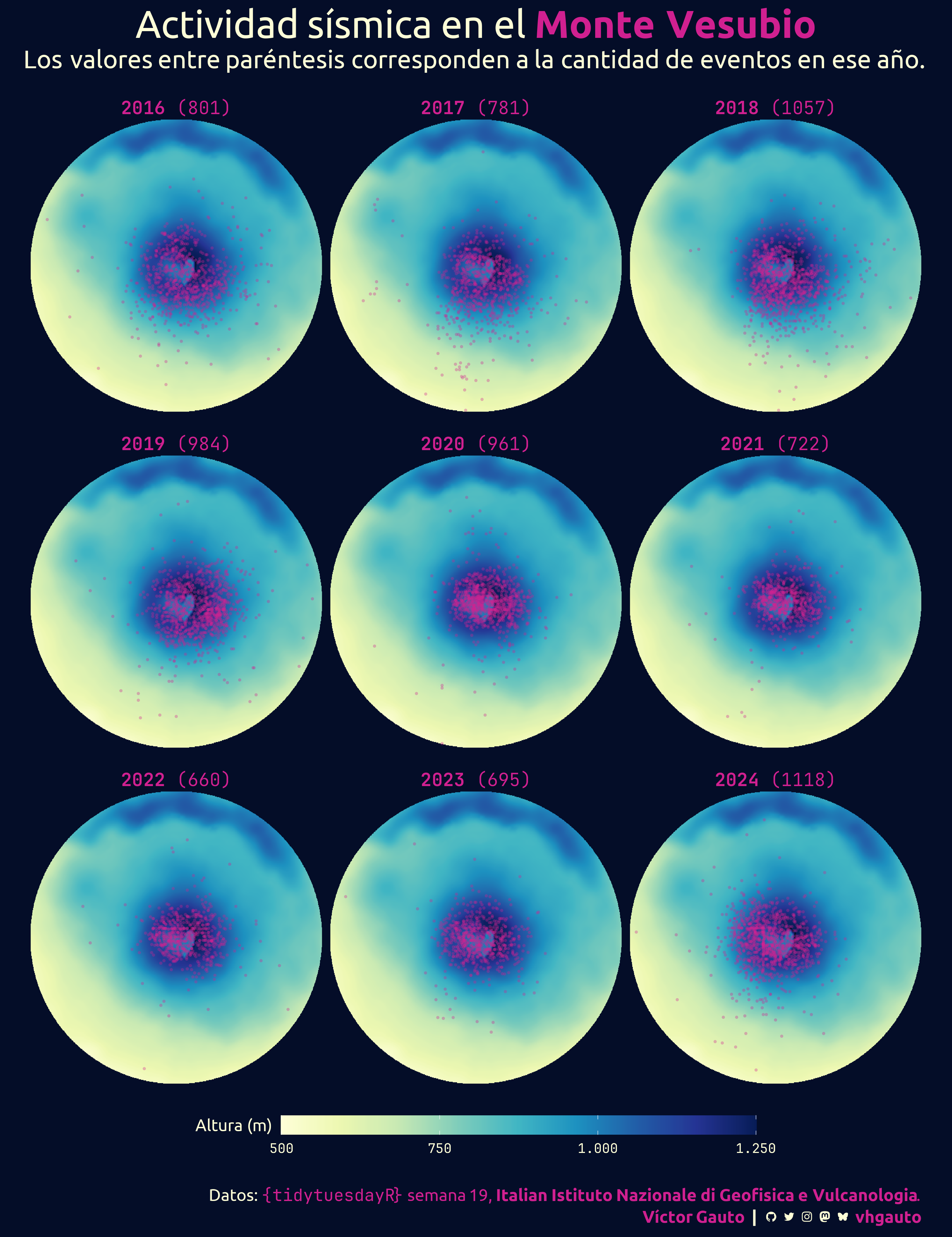
vesuvius <- tuesdata$vesuviusMe interesa la cantidad de terremotos en el Vesubio, sobre un mapa, por los últimos nueve años. El mapa es de la topografía del volcán.
Creo un vector a partir de los datos desde 2016 inclusive.
v <- vesuvius |>
  drop_na(latitude, longitude) |>
  filter(year >= 2016) |>
  terra::vect(
    geom = c("longitude", "latitude"), crs = "EPSG:4326"
  )

v_sf <- sf::st_as_sf(v)
Creo un círculo alrededor de las coordenadas del volcán y obtengo la elevación del terreno.
buf_sf <- data.frame(
  x = 14.42599167,
  y = 40.82166944
) |>
  vect(geom = c("x", "y"), crs = "EPSG:4326") |>
  buffer(2000, quadsegs = 500) |>
  sf::st_as_sf()

elev <- elevatr::get_elev_raster(
  locations = buf_sf,
  z = 13,
  clip = "locations"
) |>
  terra::rast()

names(elev) <- "altura"
Recorto los datos para conservar únicamente los que coinciden con el ráster de elevación.
v_crop <- sf::st_intersection(v_sf, buf_sf) |>
  vect()
Cuento la cantidad de eventos por año y genero etiquetas para las facetas de la figura.
v_crop_tbl <- as.data.frame(v_crop, geom = "xy") |>
  as_tibble()

v_n <- count(v_crop_tbl, year) |>
  mutate(
    label = glue("**{year}** ({n})")
  )

año_label <- v_n$label
año_label <- set_names(año_label, as.character(v_n$year))Defino un estilo para los títulos de las facetas.
label_style <- modify_style(
  classic_style(),
  "body",
  family = "JetBrains Mono",
  color = c1
)
Creo título y subtítulo.
mi_titulo <- glue(
  "Actividad sísmica en el <b style='color: {c1}'>Monte Vesubio</b>"
)

mi_subtitulo <- "Los valores entre paréntesis corresponden a la cantidad de
eventos en ese año."
Creo los mapas con los eventos sísmicos por cada año.
g <- ggplot() +
  geom_spatraster(
    data = elev, aes(fill = altura)
  ) +
  geom_spatvector(
    data = v_crop, color = c1, size = 1, alpha = 1/3, shape = 16
  ) +
  scale_fill_whitebox_c(
    palette = "deep",
    name = "Altura (m)",
    breaks = seq(500, 1250, 250),
    labels = scales::label_number(big.mark = ".", decimal.mark = ","),
    limits = c(500, 1250)
  ) +
  facet_wrap(vars(year), ncol = 3, labeller = as_labeller(año_label)) +
  coord_sf(expand = FALSE) +
  labs(title = mi_titulo, subtitle = mi_subtitulo, caption = mi_caption) +
  theme_void(base_family = "ubuntu", base_size = 15) +
  theme(
    text = element_text(color = c2),
    plot.margin = margin(r = 10, l = 10, b = 10),
    plot.background = element_rect(fill = scales::col_darker(c3), color = NA),
    plot.title = element_markdown(
      size = rel(2.3), hjust = .5, margin = margin(b = 5, t = 10)
    ),
    plot.subtitle = element_markdown(
      size = rel(1.5), hjust = .5, margin = margin(b = 10)
    ),
    plot.caption = element_markdown(
      size = rel(1), lineheight = 1.3, margin = margin(t = 30)
    ),
    strip.text = element_marquee(
      family = "jet", margin = margin(t = 10, b = 0), style = label_style,
      size = rel(1.1)
    ),
    legend.position = "bottom",
    legend.title = element_text(margin = margin(b = 18, r = 8)),
    legend.key.width = unit(3, "cm"),
    legend.box.spacing = unit(1, "cm"),
    legend.text = element_text(family = "jet")
  )
Guardo.
ggsave(
  plot = g,
  filename = "tidytuesday/2025/semana_19.png",
  width = 30,
  height = 39,
  units = "cm"
)