Ocultar código
library(sf)
library(ggrepel)
library(patchwork)
library(showtext)
library(ggtext)
library(glue)
library(tidyverse)Parques Nacionales y su extensión.
library(sf)
library(ggrepel)
library(patchwork)
library(showtext)
library(ggtext)
library(glue)
library(tidyverse)Colores.
MetBrewer::met.brewer(name = "Moreau")
c1 <- "#421600"
c2 <- "#792503"
c3 <- "white"
c4 <- "#BC7524"
c5 <- "#8DADCA"
c6 <- "#527BAA"
c7 <- "#082844"
Fuentes de texto.
font_add(
  family = "bebas",
  regular = "././fuente/BebasNeue-Regular.ttf"
)
font_add(
  family = "ubuntu",
  regular = "././fuente/Ubuntu-Regular.ttf",
  bold = "././fuente/Ubuntu-Bold.ttf",
  italic = "././fuente/Ubuntu-Italic.ttf"
)
font_add(
  family = "jet",
  regular = "././fuente/JetBrainsMonoNLNerdFontMono-Regular.ttf"
)

showtext_auto()
showtext_opts(dpi = 300)fuente <- glue(
"<b>Datos: </b> <span style='color:{c3};'>IGN</span>,
</b> <span style='color:{c3};'>Instituto Geográfico Nacional</span>"
)
autor <- glue("<span style='color:{c3};'>Víctor Gauto</span>")
icon_twitter <- glue(
"<span style='font-family:jet;'></span>"
)
icon_instagram <- glue(
"<span style='font-family:jet;'></span>"
)
icon_github <- glue(
"<span style='font-family:jet;'></span>"
)
icon_mastodon <- glue(
"<span style='font-family:jet;'>󰫑</span>"
)
icon_bluesky <- glue(
"<span style='font-family:jet;'></span>"
)
usuario <- glue("<span style='color:{c3};'>vhgauto</span>")
sep <- glue("**|**")
mi_caption <- glue(
"{fuente}<br>{autor} {sep} <b>{icon_github} {icon_twitter} ",
"{icon_instagram} {icon_mastodon} {icon_bluesky}</b> {usuario}"
)Vector de polígonos de Áreas Protegidas de Argentina, descargado del Instituto Geográfico Nacional (Geodesia y demarcación / Límites / Polígono / Área protegida).
ap <- st_read("argentina/vectores/extras/area_protegida.json") |>
  st_transform("EPSG:5346")
Conservo únicamente los Parques Nacionales. Unifico el Parque Nacional Iberá, que está dividido en varias partes.
pn <- ap |>
  filter(gna == "Parque Nacional") |>
  mutate(nam = if_else(str_detect(nam, "Iberá"), "Iberá", nam))
Combino los polígonos, calculo el áreas y recorto los nombres de los Parques Nacionales.
pn <- pn |>
  summarise(geometry = st_union(geometry), .by = nam) |>
  mutate(a = st_area(geometry)) |>
  mutate(a = as.numeric(a)) |>
  mutate(a = a * 1e-6) |>
  mutate(nam_corto = str_wrap(nam, width = 15)) |>
  mutate(nam = fct_reorder(nam, a)) |>
  mutate(nam_corto = fct_reorder(nam_corto, a)) |>
  arrange(nam) |>
  mutate(fila = row_number())
Vector de Argentina continental.
arg <- st_read("argentina/vectores/arg_continental.gpkg") |>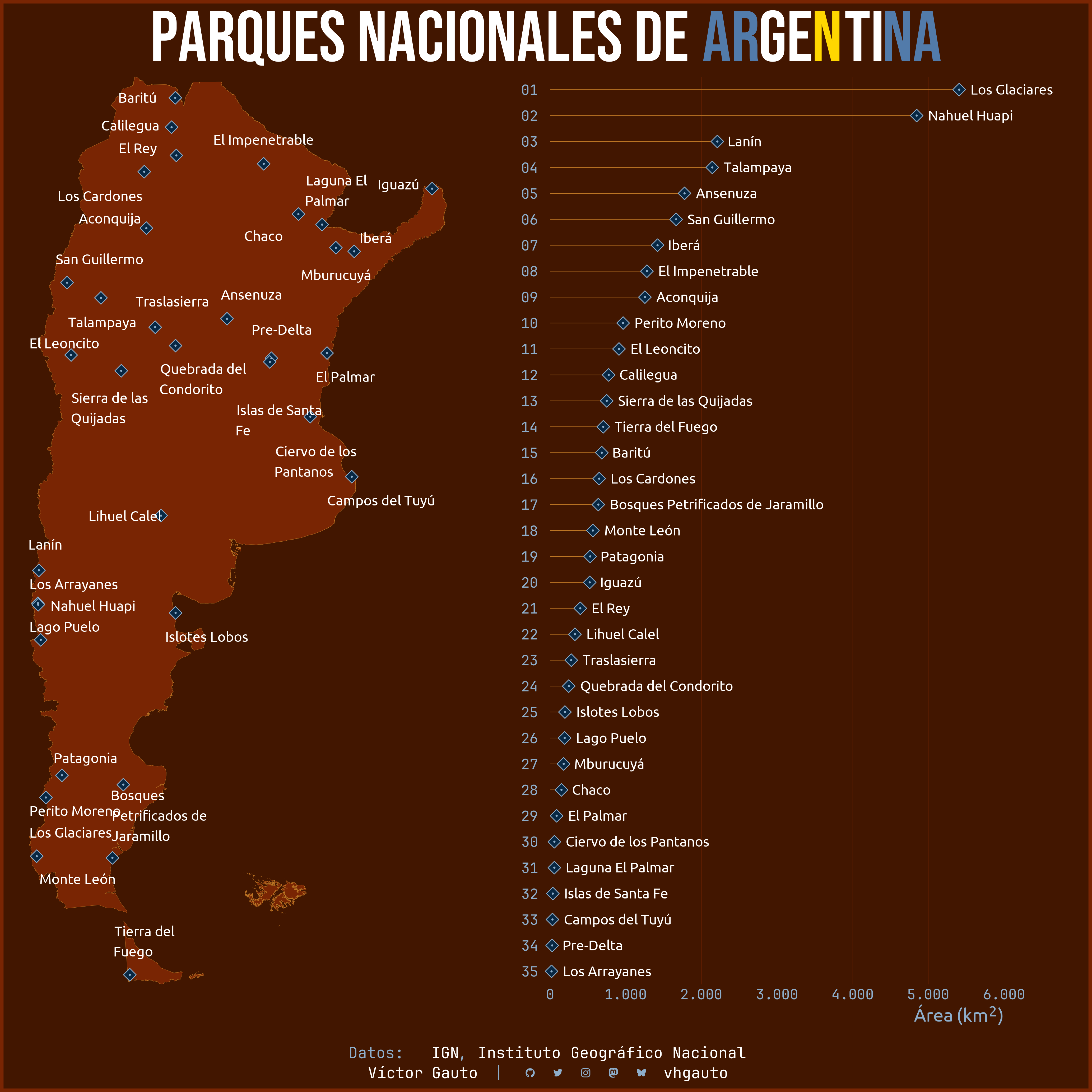
st_transform("EPSG:5346")La figura está compuesta por dos gráficos: un mapa con las ubicaciones de los Parques Nacionales y un gráfico de puntos indicando la extensión de cada uno.
Los ejes y sus títulos.
eje_x <- tibble(
  x = seq(0, 6000, 1000),
  y = 0,
  label = seq(0, 6000, 1000)
) |>
  mutate(label = format(label, big.mark = ".", decimal.mark = ","))

tit_eje_x <- tibble(
  x = 3000,
  y = -.5,
  label = "Área (km<sup>2</sup>)"
)

verticales <- tibble(
  x = seq(0, 6000, 1000),
  xend = x,
  y = .5,
  yend = nrow(pn) + .5
)
Figura de puntos.
g1 <- pn |>
  ggplot(aes(x = a, y = fila)) +
  geom_segment(
    data = verticales,
    aes(x = x, xend = xend, y = y, yend = yend),
    color = c2,
    linewidth = .1
  ) +
  geom_segment(aes(x = 0, xend = a, yend = fila), color = c4, linewidth = .25) +
  geom_point(color = c5, fill = c7, size = 4, shape = 23) +
  geom_point(shape = 16, color = c5, size = .6) +
  geom_text(
    aes(label = nam),
    nudge_x = 150,
    hjust = 0,
    color = c3,
    family = "ubuntu",
    size = 4.5
  ) +
  scale_x_continuous(
    breaks = seq(0, 6000, 1000),
    expand = c(0, 0),
    labels = scales::label_number(big.mark = ".", decimal.mark = ",")
  ) +
  scale_y_continuous(
    labels = c(nrow(pn):10, glue("0{9:1}")),
    breaks = 1:nrow(pn)
  ) +
  labs(y = NULL, x = "Área (km<sup>2</sup>)") +
  coord_cartesian(clip = "off", expand = FALSE) +
  theme_void(base_size = 13) +
  theme(
    aspect.ratio = 2,
    plot.margin = margin(10, 70, 10, 10),
    axis.title.x = element_markdown(
      family = "ubuntu",
      color = c5,
      size = rel(1.3),
      hjust = 1,
      margin = margin(t = 5)
    ),
    axis.text.x = element_text(
      family = "jet",
      color = c5,
      margin = margin(t = 3)
    ),
    axis.text.y = element_text(
      color = c5,
      family = "jet",
      hjust = 0,
      margin = margin(0, 10, 0, 0)
    ),
    axis.ticks.y = element_blank()
)Calculo los centroides de cada Parque Nacional.
cen <- pn |>
  st_centroid() |>
  st_geometry()
Mapa de los Parque Nacionales, indicando sus ubicaciones centrales. Los nombres se colocaron evitando que se superpongan mediante el paquete {ggrepel}.
g2 <- ggplot() +
  geom_sf(data = arg, fill = c2, color = c4, linewidth = .1) +
  geom_sf(data = cen, shape = 23, color = c5, fill = c7, size = 4) +
  geom_sf(data = cen, shape = 16, color = c5, size = .6) +
  geom_label_repel(
    data = pn,
    aes(label = nam_corto, geometry = geometry),
    stat = "sf_coordinates",
    size = 4.5,
    point.padding = 20,
    hjust = 0,
    family = "ubuntu",
    seed = 2025,
    fill = NA,
    color = c3,
    label.size = unit(0, "line"),
    label.padding = unit(.1, "line")
  ) +
  coord_sf(clip = "off", expand = FALSE) +
theme_void()Se combinan ambas figuras (g_col y g_sf) mediante {patchwork}.
Defino el diseño de la composición de figuras.
diseño <- "
  A#B
  A#B
"
Defino el título de la figura.
argentina <- glue(
  "<span style='color:{c6};'>Ar</span>ge<span style='color:gold;'>n</span>ti<span style='color:{c6};'>na</span>"
)

mi_titulo <- glue("Parques Nacionales de {argentina}")
Figura compuesta.
g <- g2 +
  g1 +
  plot_layout(design = diseño, widths = c(1, .1, 1)) +
  plot_annotation(
    title = mi_titulo,
    caption = mi_caption,
    theme = theme(
      plot.background = element_rect(
        fill = c1,
        color = c2,
        linewidth = 3
      ),
      plot.margin = margin(10, 10, 10, 10),
      plot.title.position = "plot",
      plot.title = element_markdown(
        hjust = .5,
        size = 65,
        family = "bebas",
        color = "white",
        margin = margin(r = -75)
      ),
      plot.caption.position = "plot",
      plot.caption = element_markdown(
        hjust = .5,
        lineheight = 1.3,
        color = c5,
        size = 14,
        family = "jet",
        margin = margin(t = 10, r = -75)
      )
    )
  )
Guardo la figura.
ggsave(
  plot = g,
  filename = "argentina/instalaciones/parques_nacionales.png",
  width = 35,
  height = 35,
  units = "cm"
)

browseURL(paste0(getwd(), "/argentina/instalaciones/parques_nacionales.png"))