Ocultar código
library(sf)
library(patchwork)
library(ggpattern)
library(ggtext)
library(glue)
library(showtext)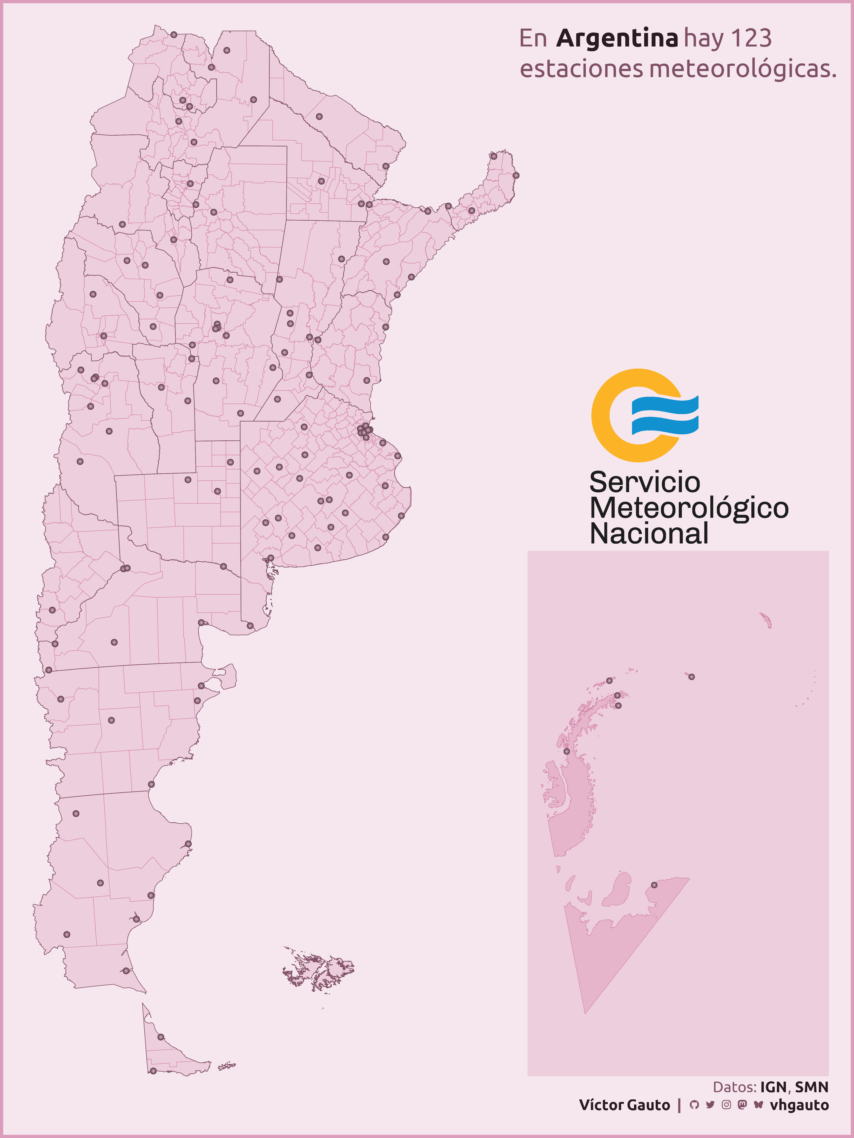
library(tidyverse)Mapa de estaciones del Servicio Meteorológico Nacional de Argentina.
library(sf)
library(patchwork)
library(ggpattern)
library(ggtext)
library(glue)
library(showtext)
library(tidyverse)Colores aleatorios a partir de una gama de rosados.
col <- monochromeR::generate_palette(
  color = "#D485AA",
  modification = "go_both_ways",
  n_colours = 9
)
Fuentes: Ubuntu y JetBrains Mono.
font_add(
  family = "ubuntu",
  regular = "././fuente/Ubuntu-Regular.ttf",
  bold = "././fuente/Ubuntu-Bold.ttf",
  italic = "././fuente/Ubuntu-Italic.ttf"
)

font_add(
  family = "jet",
  regular = "././fuente/JetBrainsMonoNLNerdFontMono-Regular.ttf"
)

showtext_auto()
showtext_opts(dpi = 300)fuente <- glue(
"Datos: <b style='color:{col[9]};'>IGN</b>, <b style='color:{col[9]};'>SMN</b>")
autor <- glue("<span style='color:{col[9]};'>**Víctor Gauto**</span>")
icon_twitter <- glue("<span style='font-family:jet;'></span>")
icon_instagram <- glue("<span style='font-family:jet;'></span>")
icon_github <- glue("<span style='font-family:jet;'></span>")
icon_mastodon <- glue("<span style='font-family:jet;'>󰫑</span>")
icon_bsky <- glue("<span style='font-family:jet;'></span>")
usuario <- glue("<span style='color:{col[9]};'>**vhgauto**</span>")
sep <- glue("**|**")
mi_caption <- glue(
"{fuente}<br>{autor} {sep} {icon_github} {icon_twitter} {icon_instagram} ",
"{icon_mastodon} {icon_bsky} {usuario}"
)Vectores de las provincias con sus departamentos. Obtengo el vector de estaciones meteorológicas del Instituto Geográfico Nacional.
p <- st_read("argentina/vectores/extras/smn_estaciones_meteorologicas.json") |>
  st_transform(crs = 5346) |>
  select(nombre)

pcias_cont <- st_read("argentina/vectores/pcias_continental.gpkg")

dptos_cont <- st_read("argentina/vectores/dptos_continental.gpkg")

dptos_antart <- st_read("argentina/vectores/dptos_antartida.gpkg")

p_cont <- st_crop(p, dptos_cont)
p_antart <- st_crop(p, dptos_antart)
Creo buffer alrededor de los puntos de las estaciones. NO pueden ser puntos para el difuminado de los colores, tiene que ser un polígono.
Como el mapa de Antártida es más pequeño, los polígonos tiene que ser más grandes.
p_cont_buffer <- st_buffer(p_cont, dist = 12000)
p_antart_buffer <- st_buffer(p_antart, dist = 30000)Logo del SMN y subtítulo de la figura.
smn <- "<img src='https://upload.wikimedia.org/wikipedia/commons/7/72/SMN_Logo_Alta.png' width='200'></img>"

mi_subtitle <- glue(
  "En <b style='color: {col[9]}'>Argentina</b> hay {nrow(p)}<br>estaciones meteorológicas.<br>"
)
Contorno del mapa y diseño de la figura compuesta.
bb <- st_bbox(pcias_cont)

diseño <- "
A#
AB
"
Mapa del sector Antártico.
g_antart <- ggplot() +
  # departamentos
  geom_sf(data = dptos_antart, fill = col[3], color = col[5]) +
  # estaciones meteorológicas
  geom_sf_pattern(
    data = p_antart_buffer, color = NA, pattern = "gradient",
    pattern_orientation = "radial",
    pattern_fill = col[3], # centro
    pattern_fill2 = col[8], # exterior
    pattern_density = 1) +
  scale_fill_viridis_d(option = "turbo") +
  coord_sf(clip = "off", expand = TRUE) +
  theme_void() +
  theme(
    plot.background = element_rect(color = NA, linewidth = 2, fill = col[2])
  )
Mapa de Argentina continental.
g_cont <- ggplot() +
  # departamentos
  geom_sf(data = dptos_cont, fill = col[2], color = col[5]) +
  # provincias
  geom_sf(data = pcias_cont, fill = NA, color = col[7], linewidth = .25) +
  # estaciones meteorológicas
  geom_sf_pattern(
    data = p_cont_buffer, color = NA, pattern = "gradient",
    pattern_orientation = "radial",
    pattern_fill = col[3], # centro
    pattern_fill2 = col[8], # exterior
    pattern_density = 1) +
  # subtítulo
  annotate(
    geom = "richtext", x = bb["xmax"], y = bb["ymax"], label = mi_subtitle,
    fill = NA, label.color = NA, hjust = 0, size = 9, color = col[7],
    family = "ubuntu", vjust = 1
  ) +
  # logo SMN
  annotate(
    geom = "richtext", x = bb["xmax"], y = 5.5e6,
    label.padding = unit(rep(1, 4), "lines"),
    label.margin = unit(rep(4, 4), "lines"),
    label = smn, fill = NA, label.color = NA, hjust = 0, vjust = 0
  ) +
  scale_fill_viridis_d(option = "turbo") +
  coord_sf(clip = "off", expand = FALSE) +
  theme_void()
Composición final del mapa.
g <- g_cont + g_antart +
  plot_layout(widths = c(1, .6), design = diseño) +
  plot_annotation(
    caption = mi_caption,
    theme = theme(
      plot.margin = margin(t = 25, r = 25, b = 25, l = 25),
      plot.background = element_rect(
        fill = col[1], color = col[4], linewidth = 3),
      plot.caption = element_markdown(
        family = "ubuntu", size = 15, color = col[7], lineheight = 1.2)
    )
  )
Guardo.
ggsave(
  plot = g,
  filename = "argentina/instalaciones/estaciones_smn.png",
  width = 30,
  height = 40,
  units = "cm"
)